Diffusion models are probabilistic generative models that define a nonlinear mapping from latent variables to the observed data.
- Like normalizing flows, the latent variables and observed data have the same dimensions.
- Like VAEs, they approximate the data likelihood using a lower bound based on an encoder that maps to the latent variable. However, in diffusion models, the encoder is pre-determined; the goal is to learn a decoder that is the inverse of this process and can be used to produce samples.
Diffusion models are easy to train and can produce very high-quality samples that exceed the realism of GANs.
Overview
A diffusion model consists of an encoder and a decoder:
- The encoder takes a data sample and maps it through a series of intermediate latent variables .
- The decoder reverses this process; it starts with and maps back through until it finally re-creates the data point .
In both the encoder and the decoder, the mappings are stochastic rather than deterministic.
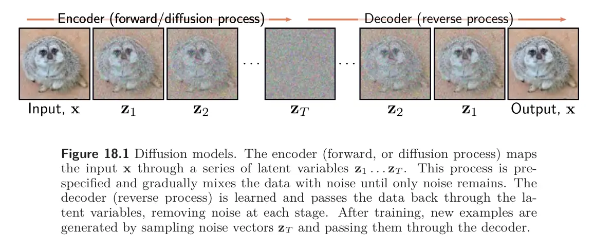
The encoder is pre-specified; it gradually blends the input with samples of white noise. With enough steps, the conditional distribution and marginal distribution of the final latent variable both become the standard normal distribution. Since this is all pre-specified, all the learned parameters are in the decoder.
In the decoder, a series of netwoks are trained to map backward between each adjacent pairs of latent variables and . The loss function encourages each network to invert the corresponding encoder step. The result is that the noise is gradually removed from the representation until a realistic-looking data example remains. To generate a new data example , we draw a sample from and pass it through the decoder.
Encoder
The Diffusion Encoder maps the data example through a series of intermediate variables:
We can find without the intermediate variables using a diffusion kernel:
Or in probabilistic form:
With this, we can marginalize to find the marginal distributions
We can also Bayes’ rule to find the conditional distribution :
but this is intractable so we just approximate it using a normal distribution.
Similarly, we can also use Bayes’ rule to find the conditional diffusion distribution :
Decoder
The Diffusion Decoder learns the reverse of the encoder. It maps from latent variables back to the data . We saw that the true reverse distributions are intractable, so we approximate them as normal distributions:
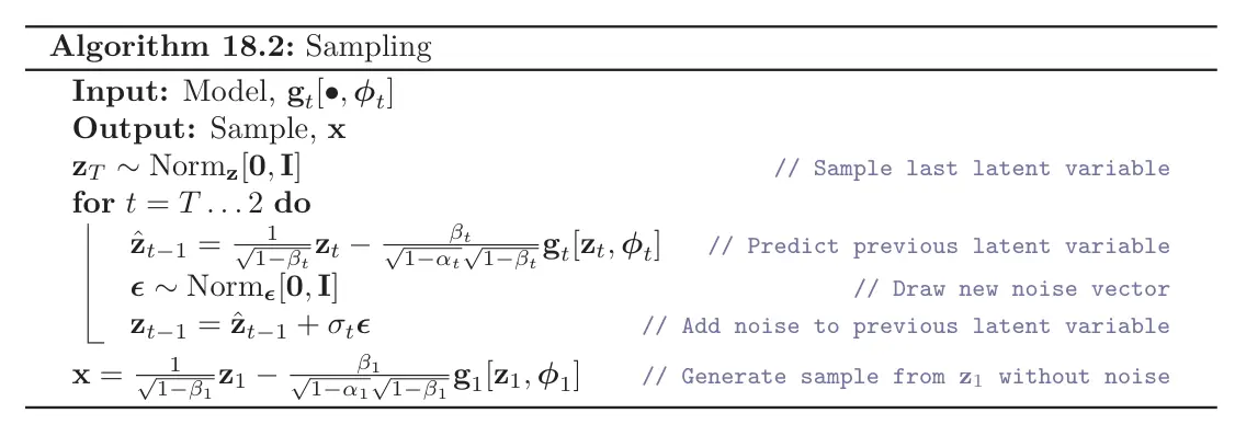
where we use a neural network to compute the mean. We can generate new samples by ancestral sampling.
Training
In Diffusion Training, we maximize the log-likelihood of the training data with respect to parameters :
However this is intractable because of . Thus, we compute an evidence lower bound (ELBO) for the log-likelihood, which ends up being:
where:
- The first term is equivalent to the reconstruction term in the VAE. The ELBO will be larger if the model prediction matches the observed data.
- The second term is the KL divergence between exact reverse posterior of the forward diffusion process , and the decoder’s learned reverse transition .
The loss function is then a minimization version of this, where we also approximate the expectations with sampling:
We then use this loss function to train a network for each diffusion timestep, minimizing the difference between the estimate of the hidden variable at the previous timestep and the most likely value that it took given the ground truth .
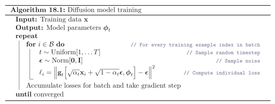
In practice, we often use a different reparameterized diffusion loss which has been found to work better. Here, the loss function is modified so that the model aims to predict the noise that was mixed with the original data example to create the current variable. It gives a simple formulation:
where we have rewritten using the diffusion kernel in the second line.
Implementation
With the reparameterized loss, we can get clean algorithms for both training and sampling:
Architecture and improvements
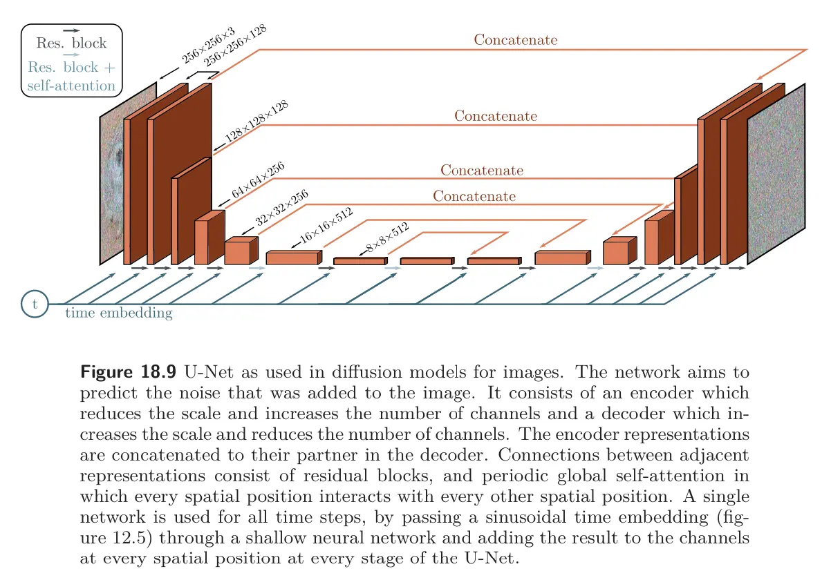
For image generation, we can use architectures such as U-Net, which are ideal for image-to-image mappings. Instead of training and storing multiple U-Nets for a large number of diffusion steps, we can instead add a time embedding.
To improve generation speed, we can use methods like DDIM, which are no longer stochastic after the first step, or accelerated sampling models, where the forward process is defined only on a subsequence of time steps. This allows the reverse process to skip timesteps, and hence makes sampling much more efficient.
For conditional generation where we have a label , we can use classifier guidance, which modifies the denoising update from to to account for . This adds a new term to the final step of the sampling algorithm that depends on the gradient of the classifier. On the other hand, classifier-free guidance avoids learning a separate classifier but instead incorporates class information into the main model , similar to how we added a time embedding before.
To improve the generation quality, we can:
- Estimate the variances in the reverse process along with the mean
- Modify the noise schedule in the forward process so that varies at each step
- Use a cascade of diffusion models: first create low-resolution images, then have subsequent models generate progressively higher-resolution images.