Normalizing Flows

Normalizing flows are probabilistic generative models, learning a probability model by transforming a simple distribution into a more complex one using a deep network. Normalizing flows can both sample from this distribution and evaluate the probability of new examples. However, they require specialized architecture; each layer must be invertible (transform data in both directions).

Normalizing flows can be used for generative applications, as well as for approximating other density models.

Intuition

See 1D Normalizing Flows Intuition for an example.

Formulation

We aim to transform a multivariate base distribution $Pr(z)$ to a model distribution $Pr(x)$ with a deep neural network.

• The invertibility requirement means that the latent space $z$ must be the same size as the data space $x$ (a continuous invertible map between ordinary Euclidean spaces requires equal dimensions).

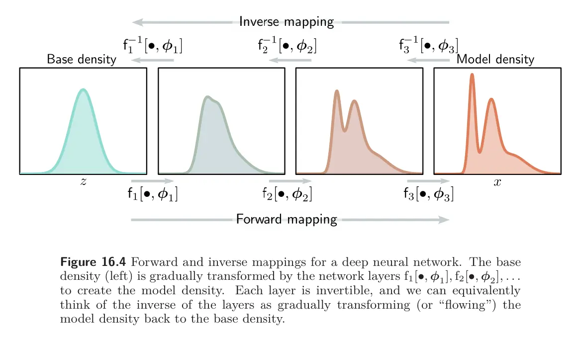
Consider applying a function $x=f[z,\varphi ]$ to a random variable $z\in {\mathbb{R}}^D$ with base density $Pr(z)$, where $f[z,\varphi ]$ is a deep network. The resulting variable $x\in {\mathbb{R}}^D$ has a new distribution. A sample $x^{\ast }$ can be drawn from this distribution by drawing a sample $z^{\ast }$ from the base density and passing it through the neural network so that $x^{\ast }=f[z^{\ast },\varphi ]$.

As we’ve seen from the 1D example, the likelihood of a sample under this distribution is:

$$Pr(x|\varphi )={\left|\frac{\partial f[z,\varphi ]}{\partial z}\right|}^{-1}\cdot Pr(z)$$

where $z=f^{-1}[x,\varphi ]$ is the latent variable $z$ that created $x$.

• The first term is the inverse of the determinant of the $D\times D$ Jacobian matrix $\partial f[z,\varphi ]/\partial z$, which contains elements $\partial f_j[z,\varphi ]/\partial z_i$ at position $(i,j)$.
  • Just as the absolute derivative measured the change of area at a point on a 1D function where the function was applied, the absolute determinant measures the change in volume at a point in the multivariate function.
• The second term is the probability of the latent variable under the base density.

Forward and inverse mapping

In practice, the forward mapping $f[z,\varphi ]$ is usually defined by a neural network, consisting of a series of layers $f_k[\bullet ,{\varphi }_k]$ with parameters ${\varphi }_k$, which are composed together as:

$$x=f[z,\varphi ]=f_K\left[f_{K-1}\right[\dots f_2[f_1[z,{\varphi }_1],{\varphi }_2],\dots {\varphi }_{K-1}],{\varphi }_K]$$

The inverse mapping (normalizing direction) is defined by the composition of the inverse of each layer $f_k^{-1}[\bullet ,{\varphi }_k]$ applied in the opposite order:

$$z=f^{-1}[x,\varphi ]=f_1^{-1}\left[f_2^{-1}\right[\dots f_{K-1}^{-1}[f_K^{-1}[x,{\varphi }_K],{\varphi }_{K-1}],\dots {\varphi }_2],{\varphi }_1]$$

The base density $Pr(z)$ is usually defined as a multivariate standard normal (i.e., with mean zero and identity covariance). Hence, the effect of each subsequent inverse layer is to gradually move or “flow” the data density toward this normal distribution. This gives rise to the name “normalizing flows”.

The Jacobian of the forward mapping can be expressed as:

$$\frac{\partial f[z,\varphi ]}{\partial z}=\frac{\partial f_1[z,{\varphi }_1]}{\partial z}\cdot \frac{\partial f_2[f_1,{\varphi }_2]}{\partial f_1}\cdot \cdots \cdot \frac{\partial f_{K-1}[f_{K-2},{\varphi }_{K-1}]}{\partial f_{K-2}}\cdot \frac{\partial f_K[f_{K-1},{\varphi }_K]}{\partial f_{K-1}}$$

where we are abusing notation to make $f_k$ the output of the function $f_k[\bullet ,{\varphi }_k]$. The absolute determinant of this Jacobian can be computed by taking the product of the individual absolute determinants:

$$\left|\frac{\partial f[z,\varphi ]}{\partial z}\right|=\left|\frac{\partial f_1[z,{\varphi }_1]}{\partial z}\right|\cdot \left|\frac{\partial f_2[f_1,{\varphi }_2]}{\partial f_1}\right|\cdot \cdots \cdot \left|\frac{\partial f_{K-1}[f_{K-2},{\varphi }_{K-1}]}{\partial f_{K-2}}\right|\cdot \left|\frac{\partial f_K[f_{K-1},{\varphi }_K]}{\partial f_{K-1}}\right|$$

The absolute determinant of the Jacobian of the inverse mapping is found by applying the same rule to the inverse mapping equation above:

$$\frac{\partial f^{-1}[x,\varphi ]}{\partial x}=\frac{\partial f_1^{-1}[f_2,\varphi ]}{\partial f_2}\cdot \frac{\partial f_2^{-1}[f_3,{\varphi }_2]}{\partial f_3}\cdot \cdots \cdot \frac{\partial f_{K-1}^{-1}[f_K,{\varphi }_{K-1}]}{\partial f_K}\cdot \frac{\partial f_K^{-1}[x,{\varphi }_K]}{\partial x}$$

The determinant can either be computed as the product of the determinants in this expression, or just the inverse of the original determinant:

$$\left|\frac{\partial f^{-1}[x,\varphi ]}{\partial x}\right|={\left|\frac{\partial f_K[f_{K-1},{\varphi }_K]}{\partial f_{K-1}}\right|}^{-1}\cdot {\left|\frac{\partial f_{K-1}[f_{K-2},{\varphi }_{K-1}]}{\partial f_{K-2}}\right|}^{-1}\dots {\left|\frac{\partial f_2[f_1,{\varphi }_2]}{\partial f_1}\right|}^{-1}\cdot {\left|\frac{\partial f_1[z,{\varphi }_1]}{\partial z}\right|}^{-1}$$

Training

We train normalizing flows with a dataset $\{x_i\}$ of $I$ training examples using the negative log-likelihood criterion:

$$\begin{array}{rl}\hat{\varphi }& =\underset{\varphi }{\mathrm{argmax}}\left[\prod _{i=1}^{I}Pr(z_i)\cdot {\left|\frac{\partial f[z_i,\varphi ]}{\partial z_i}\right|}^{-1}\right]\\ & =\underset{\varphi }{\mathrm{argmin}}\left[\sum _{i=1}^I\log \left[\left|\frac{\partial f[z_i,\varphi ]}{\partial z_i}\right|\right]-\log [Pr(z_i)]\right]\end{array}$$

where $z_i=f^{-1}[x_i,\varphi ]$, $Pr(z_i)$ is measured under the base distribution, and the determinant is calculated as above.

Architecture

The theory of normalizing flows is straightforward. However, for this to be practical, we need neural network layers $f_k$ that have four properties:

1. Collectively, the set of network layers must be sufficiently expressive to map a multivariate standard normal distribution to an arbitrary density.
2. The network layers must be invertible; each must define a unique one-to-one mapping from any input point to an output point (bijective).
3. It must be possible to compute the inverse of each layer efficiently. We need to do this every time we evaluate the likelihood. This happens repeatedly during training, so there must be a closed-form solution or a fast algorithm for the inverse.
4. It also must be possible to evaluate the determinant of the efficiently for either the forward or inverse mapping.

With these requirements in mind, we can now describe different invertible network layers or flows for use in these models. We start with linear and elementwise flows. These are easy to invert, and it’s possible to compute the determinant of their Jacobians, but neither is sufficiently expressive to describe arbitrary transformations of the base density. However, they form the building blocks of coupling, autoregressive, and residual flows, which are all more expressive.

• Linear Flows, Elementwise Flows – easy to invert and compute Jacobians, but not sufficiently expressive.
• Coupling Flows, Autoregressive Flows, Residual Flows
• Multi-scale Flows

dl
Normalizing flows
?

• Generative model where we map a base distribution $Pr(z)$ to a model distribution $Pr(x)$ with a deep neural network.
• They can both evaluate the likelihood of samples exactly and generate new samples.
• Architectural requirement: Layers must be invertible.

+++

Why do normalizing flow model layers have to be invertible?
?

• Forward transformation to generate samples
• Inverse (normalizing) transformation to evaluate likelihood of data.
• Training is done by maximizing the likelihood, requiring evaluation of the inverse transformation and its Jacobian determinant.

+++