Generative Models

Generative models map from latent variables $z$ to the data $x$. Consider defining a distribution $\text{Pr}(z)$ over the latent variable $z$ in these models. New examples can now be generated by (i) drawing from this distribution and (ii) mapping the sample to the data space $x$.

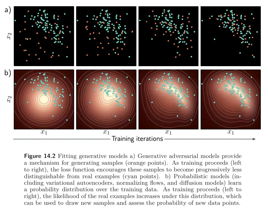
GANs learn to generate data examples $x^{\ast }$ from latent variables $z$, using a loss that encourages the generated samples to be indistinguishable from real examples.

Normalizing flows, variational autoencoders, and diffusion models are probabilistic generative models. In addition to generating new examples, they assign a probability $\text{Pr}(x|\varphi )$ to each data point $x$. This will depend on the parameters $\varphi$, and in training, we maximize the probability of the observed data $\{x_i\}$, so the loss is the sum of the negative log-likelihoods:

$$L[\varphi ]=-\sum _{i=1}^I\log [\text{Pr}(x_i|\varphi )]$$

Since probability distributions must sum to one, this implicitly reduces the probability of examples that lie far from the observed data. As well as providing a training criterion, assigning probabilities is useful in its own right:

• The probability on a test set can be used to compare two models quantitatively
• The probability for an example can be thresholded to determine if it belongs to the same dataset or is an outlier.

What makes a good generative model?

Generative models based on latent variables should have the follow properties:

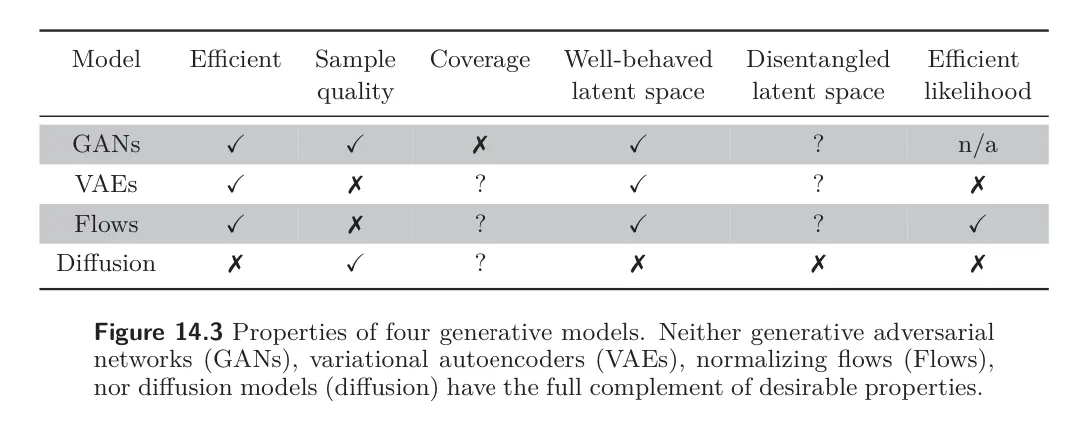
• Efficient sampling: Generating samples from the model should be computationally inexpensive and take advantage of GPU parallelism.
• High-quality sampling: The sampling should be indistinguishable from the real data with which the model was trained.
• Coverage: Samples should represent the entire training distribution. It is insufficient to generate samples that look like a subset of the training examples.
• Well-behaved latent space: Every latent variable $\mathbf{z}$ corresponds to a plausible data example $x$. Smooth changes in $\mathbf{z}$ corresponds to smooth changes in $x$.
• Disentangled latent space: Manipulating each dimension of $z$ should correspond to changing an interpretable property of the data. For example, in a model of language, it might change the topic, tense, or verbosity.
• Efficient likelihood computation: If the model is probabilistic, we would like to be able to calculate the probability of the new examples efficiently and accurately.

There is not yet a single model that satisfies all of these characteristics. Below is a subjective comparison for the methods:

Evaluation

How do we quantitatively measure the success of a generative model?

• Many of the methods are mostly used for images due to the widespread availability of data, so some of these metrics only apply to images.

Test likelihood

One way to compare probabilistic models is to measure their likelihood for a test dataset. It’s ineffective to measure the training data likelihood because a model could overfit to the training set, assigning very high probability to training points but low probabilities between them. This would result in very high training likelihood but the model can only reproduce training data instead of generating new samples. Test likelihood captures how well the model generalizes from the training data and also the coverage; if the model assigns a high probability to just a subset of the training data, it must assign lower probabilities elsewhere, which will be reflected by test likelihood as a portion of the test examples will have low probability too.

While sensible for probabilistic models, test likelihood doesn’t work for GANs which do not assign a probability. It’s also expensive to estimate for VAEs and diffusion models, although it is possible to compute a lower bound on the log-likelihood. Normalizing flows are the only type of model where test likelihood can be computed exactly and efficiently.

Inception score

The inception score (IS) is specialized for images and ideally for generative models trained on ImageNet. The score is calculated using a pre-trained classification model (Inception). It’s based on two criteria:

1. Each generated image $x^{\ast }$ should look like one of the 1000 possible classes $y$ in ImageNet. Hence, the probability distribution $Pr(y|x_i^{\ast })$ should be highly peaked at the correct class.
2. The entire set of generated images should be assigned to the classes with equal probability, so $Pr(y)$ should be flat when averaged over all generated samples.

The inception score measures the average distance between these two distributions over the generated set. This distance will be large is one is peaked and one is flat. Precisely, it returns the exponential of the KL divergence between $Pr(y|x_i^{\ast })$ and $Pr(y)$:

$$IS=\exp \left[\frac{1}{I}\sum _{i=1}^I{D}_{KL}[Pr(y|x_i^{\ast })||Pr(y)]\right]$$

where $I$ is the number of generated samples and:

$$Pr(y)=\frac{1}{I}\sum _{i=1}^{I}Pr(y|x_i^{\ast })$$

This metric is only sensible for generative models on ImageNet and is sensitive to the particular classification model. Moreover, it does not reward diversity within an object classes, returning a high value even if the model only generates one realistic example per class.

Frechet inception distance

This measure is also intended for images and computes a symmetric distance between the distributions of generated samples and real examples.

The distance must be approximate, as it is hard to characterize either distribution (characterizing the real distribution is the job of generative models in the first place). Hence, the Frechet inception distance approximates both distributions by multivariate Gaussians and estimates the distance between them using the Frechet Distance.

However, Frechet inception distance does not model the distance with respect to the original data. Rather, it uses the activations in the deepest layer of the inception classification network. These hidden units are most associated with object classes, so the comparison occurs at a semantic level, ignoring the more fine-grained details of the images.

This metric does not take account of diversity within classes but relies heavily on the information retained by the features in the inception network. Any information discarded by the network does not contribute to the result. Some this is discarded information may still be important to generate realistic examples.

Manifold precision/recall

Frechet inception distance is sensitive to both the diversity and the realism of the generated samples but doesn’t distinguish between these two factors. To disentangle these qualities, we consider the overlap between the data manifold (the subset of the data space where real examples lie) and the model manifold (the subset of the data space where generated samples lie). The precision is the fraction of the model samples that are realistic. The recall is the fraction of data examples that fall within the model manifold. This measures the proportion of real data the model can generate.

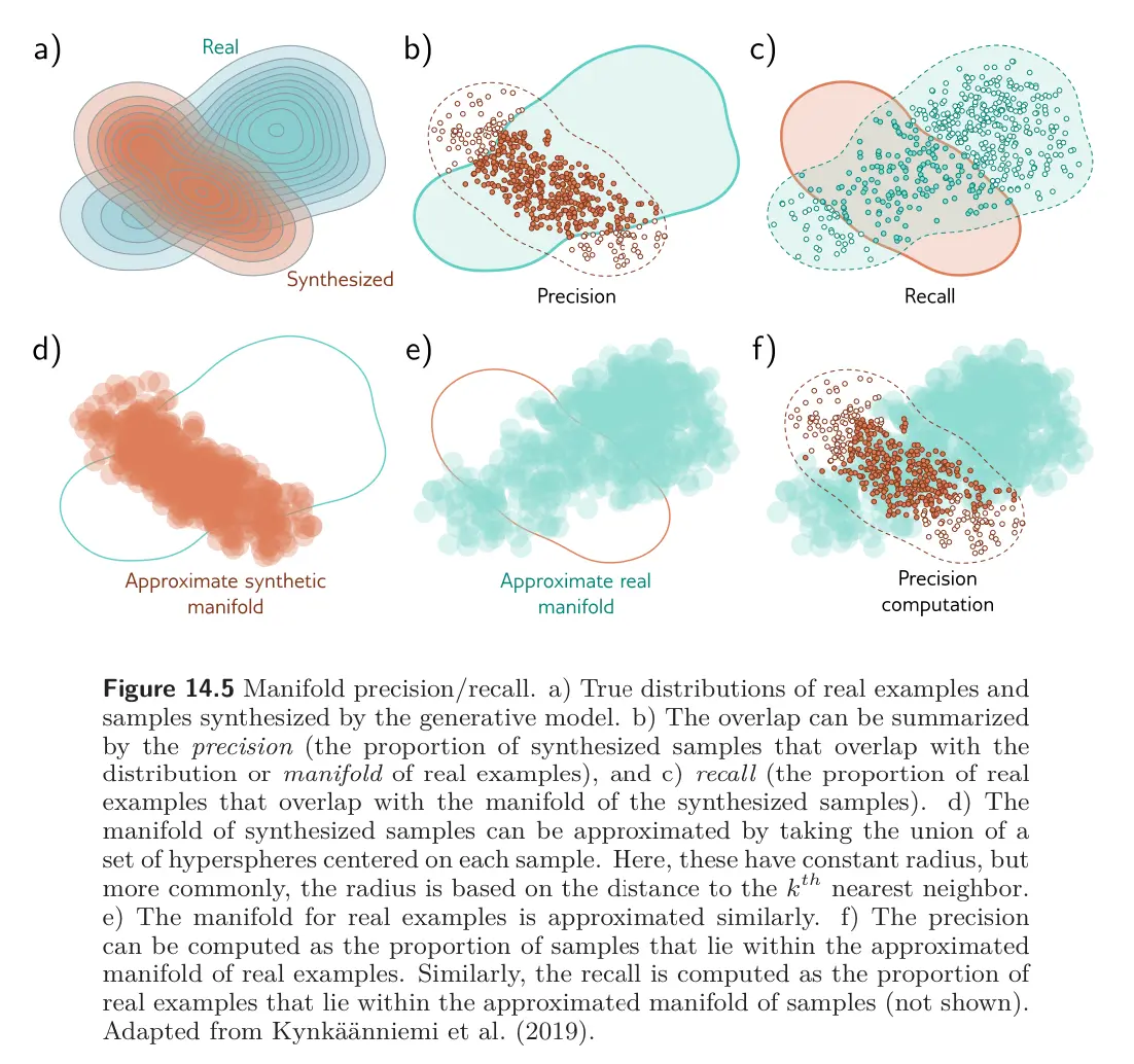
To estimate the manifold, we place a hypersphere around each data example, whose radius is the distance to the $k$-th nearest neighbor. The union of these spheres is an approximation of the manifold, and it’s easy to determine if a new point lies within it. This manifold is also typically computed in the feature space of a classifier (with the advantages and disadvantages that entails).