Variational Autoencoder

Variational autoencoders are probabilistic generative models; they aim to learn a distribution $Pr(x)$ over the data. After training, we can draw (generate) samples from this distribution. However, unlike normalizing flows, VAEs cannot evaluate the probability of new samples $x^{\ast }$ exactly, although we can approximate it using importance sampling.

Note that the VAE is not the model of $Pr(x)$; it is the neural architecture that is designed to learn the model for $Pr(x)$. The final model for $Pr(x)$ contains neither the “variational” nor the “autoencoder” parts and might be better described as a nonlinear latent variable model, where we model a joint distribution $Pr(x,z)$ of the data $x$ and an unobserved hidden or latent variable $z$.

Specifically, we use:

• A prior distribution $Pr(z)$ over the latent variable.
• A network $f[z,\varphi ]$ that maps a latent to the data space (decoder).

Then, the likelihood (conditional to $z$) can be found as

$$Pr(x|z,\varphi )={\text{Norm}}_x[f[z,\varphi ],{\sigma }^{2}I]$$

which can then be marginalized over $z$ to get the data probability:

$$\begin{array}{rl}Pr(x|\varphi )& =\int Pr(x,z|\varphi )dz\\ & =\int Pr(x|z,\varphi )\cdot Pr(z)dz\\ & =\int {\text{Norm}}_x[f[z,\varphi ],{\sigma }^{2}I]\cdot {\text{Norm}}_z[0,I]dz\end{array}$$

ELBO Objective

To train the model, we maximize the log-likelihood over a training dataset $\{x_i{\}}_{i=1}^I$ with respect to the model parameters. For simplicity, we assume that the variance term ${\sigma }^2$ in the likelihood expression is known and concentrate on learning $\varphi$:

$$\hat{\varphi }=\underset{\varphi }{\mathrm{argmax}}\left[\sum _{i=1}^I\log [Pr(x_i|\varphi )]\right]$$

where

$$Pr(x_i|\varphi )=\int {\text{Norm}}_{x_i}[f[z,\varphi ],{\sigma }^{2}I]\cdot {\text{Norm}}_z[0,I]dz$$

Unfortunately, this is intractable. There is no closed-form expression for the integral and no easy way to evaluate it for a particular value of $x$.

To make progress, we define a lower bound on the log-likehood $\log [Pr(x_i|\varphi )]$ with ELBO. Given some distribution $q(z)$ with parameters $\theta$, the ELBO can be written in 3 forms:

$$\begin{array}{rl}\text{ELBO}[\theta ,\varphi ]& =\int q(z|\theta )\log \left[\frac{Pr(x,z|\varphi )}{q(z|\theta )}\right]dz\\ & =\log [Pr(x|\varphi )]-D_{KL}[q(z|\theta )||Pr(z|x,\varphi )]\\ & =\int q(z|\theta )\log [Pr(x|z,\varphi )]dz-D_{KL}[q(z|\theta )\left|\right|Pr(z)]\end{array}$$

• The first form is a naive derivation from Jensen’s Inequality
• The second form shows that ELBO is equal to the log-likelihood (tight) when $q(z|\theta )=Pr(z|x,\varphi )$
• The third form expresses ELBO in terms of a reconstruction accuracy between the latent variable and the data (first term) and the similarity between the auxiliary distribution $q(z|\theta )$ and the prior.

To learn the nonlinear latent variable model, we maximize this quantity as a function of both $\varphi$ and $\theta$. The neural architecture that computes this quantity is the VAE.

Variational approximation

We saw that ELBO tight when $q(z|\theta )$ is the posterior $Pr(z|x,\varphi )$. In principle, we can compute the posterior using Bayes’ rule:

$$Pr(z|x,\varphi )=\frac{Pr(x|z,\varphi )Pr(z)}{Pr(x|\varphi )}$$

This is unfortunately also intractable because we can’t evaluate the evidence term $Pr(x|\varphi )$ in the denominator.

One solution is to make a variational approximation: we choose a simple parametric form for $q(z|\theta )$ and use this to approximate the true posterior $Pr(z|x,\varphi )$. Here, we choose a multivariate normal distribution with mean $\mu$ and diagonal covariance $\Sigma$. This will not always match the posterior well, but will be better for some values of $\mu$ and $\Omega$ than others. During training, we will find the normal distribution that is “closest” to the true posterior, which conceptually corresponds to minimizing the KL divergence in the second form of ELBO above. We cannot evaluate this posterior KL directly because the true posterior is intractable; instead, we maximize the algebraically equivalent reconstruction-minus-prior-KL form of ELBO (third form above) to train as we can use the known prior $Pr(z)$.

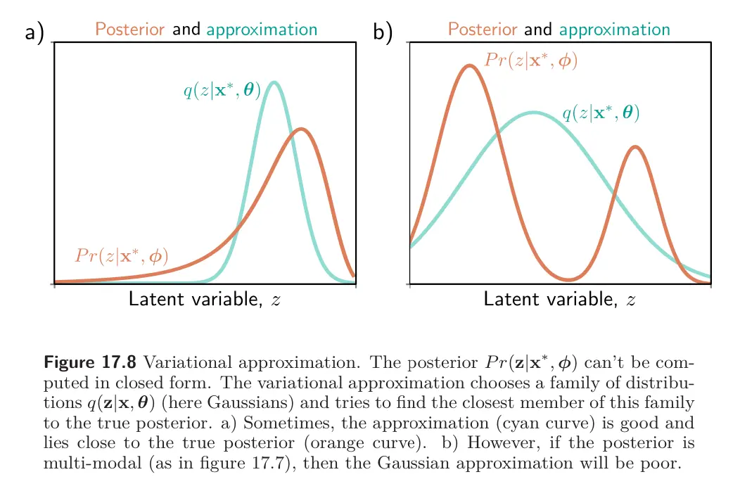
Since the optimal choice for $q(z|\theta )$ was the posterior $Pr(z|x)$, and this depends on the data example $x$, the variational approximation should do the same, so we choose:

$$q(z|x,\theta )={\text{Norm}}_z[g_{\mu }[x,\theta ],g_{\Sigma }[x,\theta ]]$$

where $g[x,\theta ]$ is a second neural network (encoder) with parameters $\theta$ that predicts the mean $\mu$ and variance $\Sigma$ of the normal variational approximation.

VAE Formulation

Finally, we can describe the VAE. We build a network that computes the third form of ELBO:

$$\text{ELBO}[\theta ,\varphi ]=\int q(z|x,\theta )\log [Pr(x|z,\varphi )]dz-D_{KL}[q(z|x,\theta )\left|\right|Pr(z)]$$

where the distribution $q(z|x,\theta )$ is the approximation from above.

The first term still involves an intractable integral, but since it is an expectation with respect to $q(z|x,\theta )$, we can approximate it by sampling. For any function $a[\bullet ]$ we have:

$${\mathbb{E}}_z[a[z]]=\int a[z]q(z|x,\theta )dz\approx \frac{1}{N}\sum _{n=1}^{N}a[z_n^{\ast }]$$

where $z_n^{\ast }$ is the $n$-th sample from $q(z|x,\theta )$. This is known as the Monte Carlo estimate.

For a very approximate estimate, we can just use a single sample $z^{\ast }$ from $q(z|x,\theta )$:

$$\boxed{\text{ELBO}[\theta ,\varphi ]\approx \log [Pr(x|z^{\ast },\varphi )]-D_{KL}[q(z|x,\theta )||Pr(z)]}$$

The second term is the KL divergence between the variational distribution $q(z|x,\theta )={\text{Norm}}_z[\mu ,\Sigma ]$ and the prior $Pr(z)={\text{Norm}}_z[0,I]$. The KL divergence between two normal distributions can be calculated in closed form. In this case, one of the distributions has parameters $\mu ,\Sigma$ and the other is a standard normal, giving us

$$D_{KL}[q(z|x,\theta )\left|\right|Pr(z)]=\frac{1}{2}(\text{Tr}\left|\Sigma \right|+{\mu }^T\mu -D_z-\log [\det \left|\Sigma \right|])$$

where $D_z$ is the dimensionality of the latent space.

Architecture

So, we want to build a model that computes the evidence lower bound for a point $x$. Then we use an optimization algorithm to maximize this lower bound over the dataset and hence improve the log-likelihood.

To compute the ELBO we:

• Compute the mean $\mu$ and variance $\Sigma$ of the variational posterior distribution $q(z|\theta ,x)$ for this data point $x$ using the network $g[x,\theta ]$.
• Draw a sample $z^{\ast }$ from the distribution.
• Compute the ELBO using the boxed equation above.

The associated architecture is shown below.

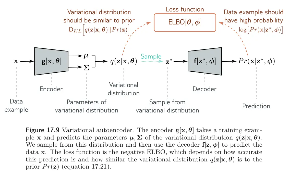
This architecture is:

• Variational because it computes a Gaussian approximation to the posterior distribution.
• Autoencoder because it starts with a data point $x$, computes a lower-dimensional latent vector $z$ from this, and then uses this to vector to recreate the data point $x$ as closely as possible.
  • The mapping from the data to the latent variable by the network $g[z,\theta ]$ is called the encoder.
  • The mapping from the latent variable to the data by the network $f[z,\varphi ]$ is called the decoder.

The VAE computes the ELBO as a function of both $\varphi$ and $\theta$. To maximize this bound, we run mini-batches of samples through the network and update these parameters with an optimization algorithm such as SGD or Adam. The gradients of the ELBO with respect to the parameters are computed as usual using automatic differentiation. During this process, we are both moving between the colored curves (changing $\theta$) and along them (changing $\varphi$). During this process, the parameters $\varphi$ change to assign the data a higher likelihood in the nonlinear latent variable model.

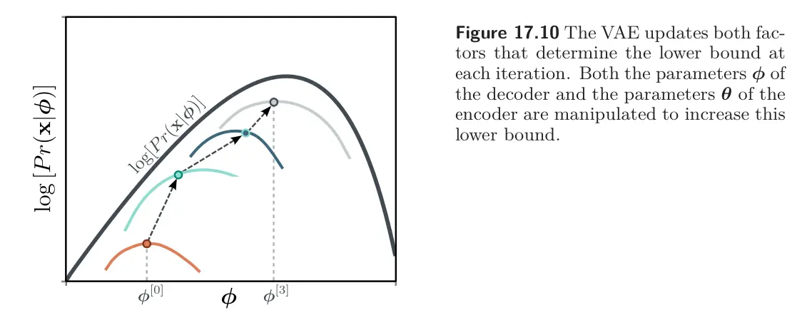
• The encoder approximates the posterior distribution over the latent variables to make the bound tight, and the decoder maximizes this bound.

Reparameterization trick

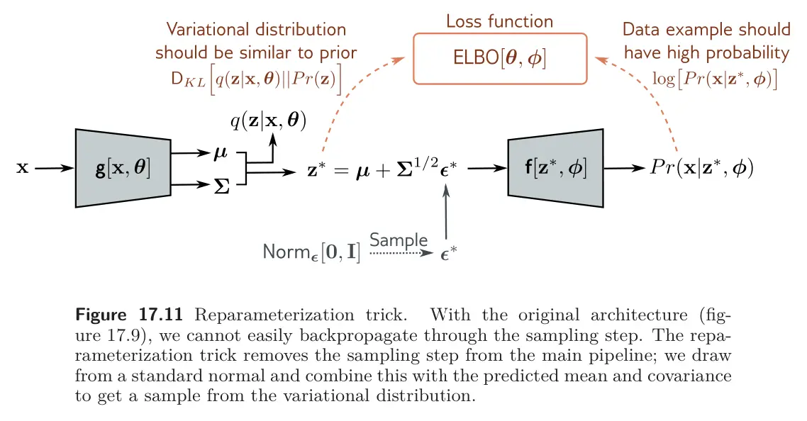
The network involves a sampling step, and it is difficult to differentiate through this stochastic component. However, we need to differentiate past this step to update the parameters $\theta$ that precede it in the network.

Fortunately, there is a simple solution; we move the stochastic part into a branch of the network that draws from a sample ${ϵ}^{\ast }$ from ${\text{Norm}}_e[0,I]$ and then use the relation:

$$z^{\ast }=\mu +{\Sigma }^{1/2}{ϵ}^{\ast }$$

to draw from the intended Gaussian. Now, we can compute the derivatives as usual because the backpropagation algorithm does not need to pass down the stochastic branch. This is known as the reparameterization trick.

Sampling

To sample from a VAE, we can simply draw from the prior $Pr(z)$ over the latent variable, pass the result through the decoder, and add noise according to $Pr(x|f[z,\varphi ])$. In practice, for high-quality generation, we want to use some tricks.

dl
How do you generate new samples with a VAE?::Sample from the latent prior distribution, pass the result through the decoder, and add independent Gaussian noise.

For VAE training, how do we deal with not being able to get exact likelihood of a data point?::The exact likelihood being intractable poses problems for training with maximum likelihood. Thus, we define a lower bound (ELBO) and maximize this bound.

What is the variational posterior approximation in a VAE?::For the ELBO bound to be tight, we need to compute the posterior probability of the latent variable given the observed data $Pr(z|x,\varphi )$. This is unfortunately also intractable, so we use the variational approximation – a simpler distribution (Gaussian) that approximates the posterior, whose parameters are computed by the encoder network.