Diffusion Training

In a diffusion model:

• The encoder maps the data example $x$ through a series of intermediate variables $z_1,z_2,\dots ,z_T$, adding noise.
• The decoder learns a series of probabilistic mappings back from latent variable $z_T$ to $z_{T-1}$, from $z_{T-1}$ to $z_{T-2}$, and so on, until we reach the data $x$.

The joint distribution of the observed variable $x$ and the latent variables $\{z_t\}$ is:

$$Pr(x,z_{1\dots T}|{\varphi }_{1\dots T})=Pr(x|z_1,{\varphi }_1)\prod _{t=2}^{T}Pr(z_{t-1}|z_t,{\varphi }_t)\cdot Pr(z_T)$$

The likelihood of the observed data $Pr(x|{\varphi }_{1\dots T})$ is found by marginalizing over the latent variables:

$$Pr(x|{\varphi }_{1\dots T})=\int Pr(x,z_{1\dots T}|{\varphi }_{1\dots T})d{z}_{1\dots T}$$

To train the model, we maximize the log-likelihood of the training data $\{x_i\}$ with respect to parameters $\varphi$:

$${\hat{\varphi }}_{1\dots T}=\underset{{\varphi }_{1\dots T}}{\mathrm{argmax}}\left[\sum _{i=1}^J\log [Pr(x_i|{\varphi }_{1\dots T})]\right]$$

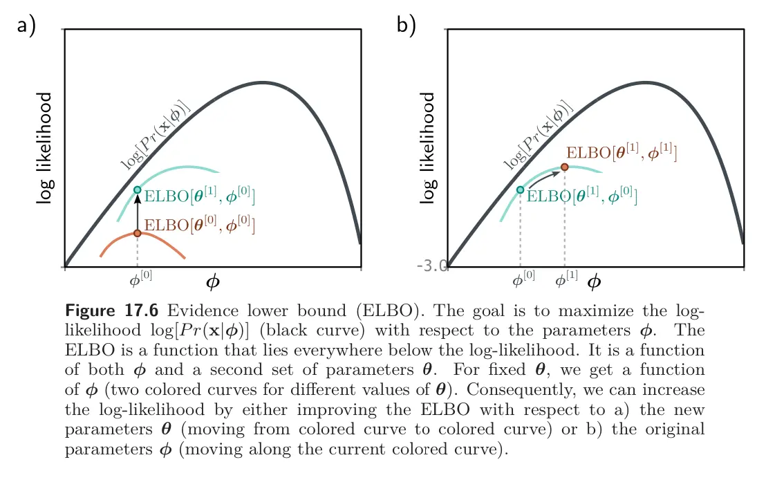
We can’t maximize this directly because the marginalization in the equation above is intractable. Hence, we use Jensen’s inequality to define a lower bound on the likelihood and optimize the parameters ${\varphi }_{1\dots T}$ with respect to this bound exactly as we did for the VAE.

Evidence lower bound (ELBO)

To derive the lower bound, we multiply and divide the log-likelihood by the encoder distribution $q(z_{1\dots T}|x)$ and apply Jensen’s Inequality:

$$\begin{array}{rl}\log [Pr(x|{\varphi }_{1\dots T})]& =\log \left[\int Pr(x,z_{1\dots T}|{\varphi }_{1\dots T})d{z}_{1\dots T}\right]\\ & =\log \left[\int q(z_{1\dots T}|x)\frac{Pr(x,z_{1\dots T}|{\varphi }_{1\dots T})}{q(z_{1\dots T}|x)}d{z}_{1\dots T}\right]\\ & \ge \int q(z_{1\dots T}|x)\log \left[\frac{Pr(x,z_{1\dots T}|{\varphi }_{1\dots T})}{q(z_{1\dots T}|x)}\right]d{z}_{1\dots T}\end{array}$$

This gives us the evidence lower bound (ELBO):

$$\text{ELBO}[{\varphi }_{1\dots T}]=\int q(z_{1\dots T}|x)\log \left[\frac{Pr(x,z_{1\dots T}|{\varphi }_{1\dots T})}{q(z_{1\dots T}|x)}\right]d{z}_{1\dots T}$$

In the VAE, the encoder $q(z|x)$ approximates the posterior distribution over the latent variables to make the bound tight, and the decoder maximizes this bound. In a diffusion model, the decoder does all the work because the encoder has no parameters. It makes the bound tighter by (i) changing its parameters so that the static encoder does approximate the posterior $Pr(z_{1\dots T}|x,{\varphi }_{1\dots T})$ and (ii) optimizing its own parameters with respect to the bound.

Simplifying ELBO

Let’s manipulate the log term from ELBO into the final form that we will optimize. First, we substitute the joint distributions for $Pr(x,z_{1\dots T}|{\varphi }_{1\dots T})$ and $q(z_{1\dots T}|x)$:

$$\begin{array}{rl}\log \left[\frac{Pr(x,z_{1\dots T}|{\varphi }_{1\dots T})}{q(z_{1\dots T}|x)}\right]& =\log \left[\frac{Pr(x|z_1,{\varphi }_1){\prod }_{t=2}^{T}Pr(z_{t-1}|z_t,{\varphi }_t)\cdot Pr(z_T)}{q(z_1|x){\prod }_{t=2}^{T}q(z_t|z_{t-1})}\right]\\ & =\log \left[\frac{Pr(x|z_1,{\varphi }_1)}{q(z_1|x)}\right]+\log \left[\frac{{\prod }_{t=2}^{T}Pr(z_{t-1}|z_t,{\varphi }_t)}{{\prod }_{t=2}^{T}q(z_t|z_{t-1})}\right]+\log [Pr(z_T)]\end{array}$$

Then we expand the denominator of the second term:

$$q(z_t|z_{t-1})=q(z_t|z_{t-1},x)=\frac{q(z_{t-1}|z_t,x)q(z_t|x)}{q(z_{t-1}|x)}$$

where:

• The first equality follows because all of the information about variable $z_t$ is encompassed in $z_{t-1}$, so the extra conditioning on the data $x$ is irrelevant.
• The second equality is a straightforward application of Bayes’ rule.

Substituting in this result gives:

$$\begin{array}{rl}\log \left[\frac{Pr(x,z_{1\dots T}|{\varphi }_{1\dots T})}{q(z_{1\dots T}|x)}\right]& =\log \left[\frac{Pr(x|z_1,{\varphi }_1)}{q(z_1|x)}\right]+\log \left[\frac{{\prod }_{t=2}^{T}Pr(z_{t-1}|z_t,{\varphi }_t)\cdot q(z_{t-1}|x)}{{\prod }_{t=2}^{T}q(z_t|z_{t-1})\cdot q(z_t|x)}\right]+\log [Pr(z_T)]\\ & =\log [Pr(x|z_1,{\varphi }_1)]+\log \left[\frac{{\prod }_{t=2}^{T}Pr(z_{t-1}|z_t,{\varphi }_t)}{q(z_{t-1}|z_t,x)}\right]+\log \left[\frac{Pr(z_t)}{q(z_T|x)}\right]\\ & \approx \log [Pr(x|z_1,{\varphi }_1)]+\sum _{t=2}^T\log \left[\frac{Pr(z_{t-1}|z_t,{\varphi }_t)}{q(z_{t-1}|z_t,x)}\right]\end{array}$$

where all but two of the terms in the product of the ratios $q(z_{t-1}|x)/q(z_t|x)$ cancel out between lines 2 and 3, leaving only $q(z_1|x)$ and $q(z_T|x)$. The last term in the third line is approximately $\log [1]=0$ since the result of the forward process $q(z_T|x)$ is a standard normal distribution, and so is equal to the prior $Pr(z_T)$.

Hence, the simplified ELBO is:

$$\begin{array}{rl}\text{ELBO}[{\varphi }_{1\dots T}]& =\int q(z_{1\dots T}|x)\log \left[\frac{Pr(x,z_{1\dots T}|{\varphi }_{1\dots T})}{q(z_{1\dots T}|x)}\right]d{z}_{1\dots T}\\ & \approx \int q(z_{1\dots T})\left(\log [Pr(x|z_1,{\varphi }_1)]+\sum _{t=2}^n\log \left[\frac{Pr(z_{t-1}|z_t,{\varphi }_t)}{q(z_{t-1}|z_t,x)}\right]\right)d{z}_{1\dots T}\\ & ={\mathbb{E}}_{q(z_1|x)}[\log [Pr(x|z_1,{\varphi }_1)]]-\sum _{t=2}^T{\mathbb{E}}_{q(z_{t,t-1}|x)}[D_{KL}[q(z_{t-1}|z_t,x)\mid \mid Pr(z_{t-1}|z_t,{\varphi }_t)]]\end{array}$$

where we have marginalized over the irrelevant variables in $q(z_{1\dots T}|x)$ between lines 2 and 3 and used the definition of KL divergence.

Analyzing ELBO

The first term in the ELBO was defined previously in the decoder:

$$Pr(x|z_1,{\varphi }_1)={\text{Norm}}_x[f_1[z_1,{\varphi }_1],{\sigma }_1^{2}I]$$

and is equivalent to the reconstruction term in the VAE. The ELBO will be larger if the model prediction matches the observed data. Like the VAE, we will approximate the expectation over the log of this quantity using a Monte Carlo estimate, in which we estimate the expectation with a sample from $q(z_1|x)$.

The KL divergence in the ELBO measures the distance between $Pr(z_{t-1}|z_t,{\varphi }_t)$ and $q(z_{t-1}|z_t,x)$, which were also defined previously in the encoder and decoder:

$$\begin{array}{rl}Pr(z_{t-1}|z_t,{\varphi }_t)& ={\text{Norm}}_{z_{t-1}}[f_t[z_t,{\varphi }_t],{\sigma }_t^{2}I]\\ q(z_{t-1}|z_t,x)& ={\text{Norm}}_{z_{t-1}}\left[\frac{(1-{\alpha }_{t-1})}{1-{\alpha }_t}\sqrt{1-{\beta }_t}{z}_t+\frac{\sqrt{{\alpha }_{t-1}{\beta }_t}}{1-{\alpha }_t}x,\frac{{\beta }_t(1-{\alpha }_{t-1})}{1-{\alpha }_t}I\right]\end{array}$$

The KL divergence between two normal distributions has a closed-form expression. Moreover, many of the terms in this expression do not depend on $\varphi$, and the expression simplifies to the squared difference between the means plus a constant $C$:

$$D_{KL}[q(z_{t-1}|z_t,x)\mid \mid Pr(z_{t-1}|z_t,{\varphi }_t)]=\frac{1}{2{\sigma }_t^2}{\left|\left|\frac{(1-{\alpha }_{t-1})}{1-{\alpha }_t}\sqrt{1-{\beta }_t}{z}_t+\frac{\sqrt{{\alpha }_{t-1}}{\beta }_t}{1-{\alpha }_t}x-f_t[z_t,{\varphi }_t]\right|\right|}^2+C$$

Diffusion loss function

To fit the model, we maximize the ELBO with respect to the parameters ${\varphi }_{1\dots T}$. We recast this as a minimization by multiplying with minus one and approximating the expectations with samples to give the loss function:

$$\begin{array}{r}L[{\varphi }_{1\dots T}]=\sum _{i=I}^I\left(\underset{\text{reconstruction term}}{\underbrace{-\log [{\text{Norm}}_{x_i}[f_1[z_{i_1},{\varphi }_1],{\sigma }_1^{2}I]]}}+\sum _{t=2}^T\frac{1}{2{\sigma }_t^2}{\left|\left|\underset{\text{target, mean of }q(z_{t-1}|z_t,x)}{\underbrace{\frac{1-{\alpha }_{t-1}}{1-{\alpha }_t}\sqrt{1-{\beta }_t}{z}_{it}+\frac{\sqrt{{\alpha }_{t-1}{\beta }_t}}{1-{\alpha }_t}{x}_i}}-\underset{\text{predicted }{z}_{t-1}}{\underbrace{f_t[z_{it},{\varphi }_t]}}\right|\right|}^2\right)\end{array}$$

where $x_i$ is the $i$-th data point, and $z_{it}$ is the associated latent variable at diffusion step $t$.

Although this loss function can be used, diffusion models have been found to work better with a reparameterized version.

Training procedure

This loss function can be used to train a network for each diffusion time step. It minimizes the difference between the estimate $f_t[z_t,{\varphi }_t]$ of the hidden variable at the previous time step and the most likely value that it took given the ground truth de-noised data $x$.

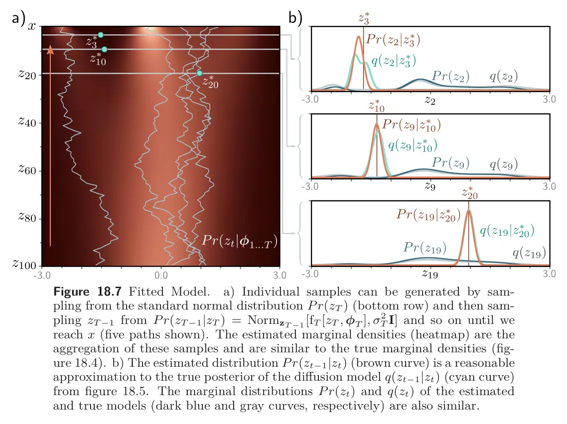
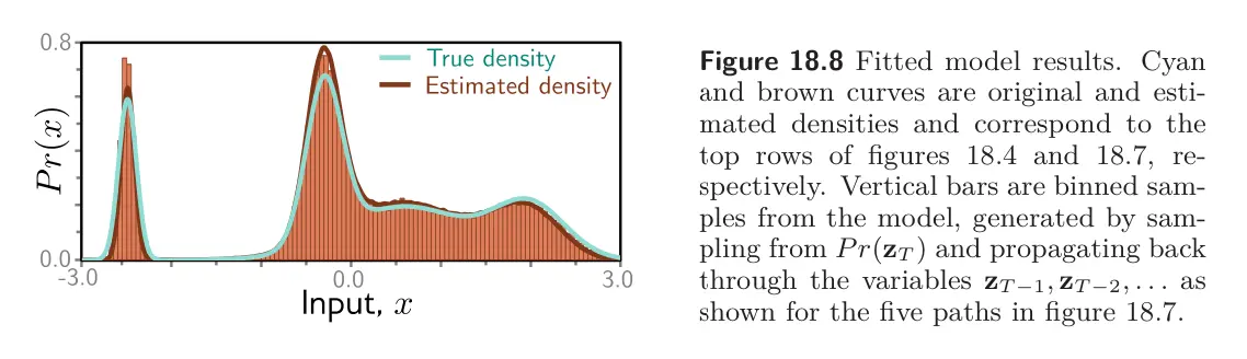
The figures below show the fitted reverse process for a simple 1D example. This model was trained by:

1. Taking a large dataset of examples $x$ from the original density
2. Using the diffusion kernel to predict many corresponding values for the latent variable $z_t$ at each time $t$
3. Training the models $f_t[z_t,{\varphi }_t]$ to minimize the loss function above.