Diffusion Encoder

In a diffusion model, the diffusion or forward process maps a data example $x$ through a series of intermediate variables $z_1,z_2,\dots ,z_T$.

• Note that this is opposite nomenclature to normalizing flows, where the inverse mapping moves from the data to the latent variable.

The mapping is done according to

$$\begin{array}{rl}{z}_1& =\sqrt{1-{\beta }_1}\cdot x+\sqrt{{\beta }_1}\cdot {ϵ}_1\\ z_t& =\sqrt{1-{\beta }_t}\cdot z_{t-1}+\sqrt{{\beta }_t}\cdot {ϵ}_t\forall t\in 2,\dots ,T\end{array}$$

where ${ϵ}_t$ is drawn from a standard normal distribution.

• The first term attenuates the data plus any noise added so far
• The second term adds more noise
• The hyperparameters ${\beta }_t\in [0,1]$ determine how quickly the noise is blended and are collectively known as the noise schedule.

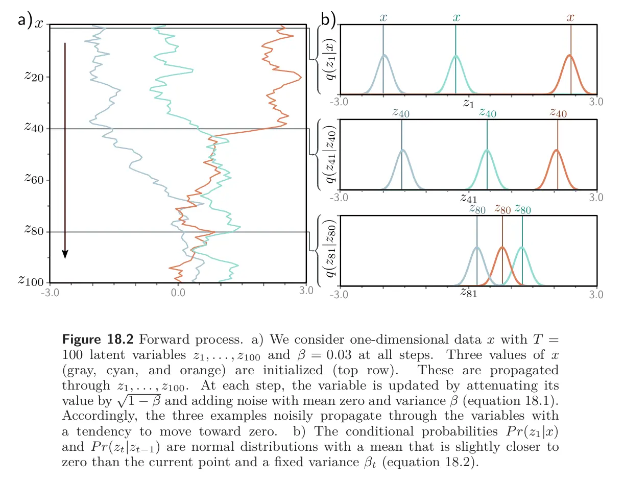
The forward process can be equivalently written as:

$$\begin{array}{rl}q(z_1|x)& ={\text{Norm}}_{z_1}[\sqrt{1-{\beta }_1}x,{\beta }_{1}I]\\ q(z_t|z_{t-1})& ={\text{Norm}}_{z_t}[\sqrt{1-{\beta }_t}{z}_{t-1},{\beta }_{t}I]\forall t\in \{2,\dots ,T\}\end{array}$$

This is a Markov Chain because the probability $z_t$ is determined entirely by the value of the immediately preceding valuable $z_{t-1}$. With sufficient steps $T$, all traces of the original data are removed, and $q(z_T|x)=q(z_T)$ becomes a standard normal distribution.

The joint distribution of all latent variables $z_1,z_2,\dots ,z_T$ given input $x$ is:

$$q(z_{1\dots T}|x)=q(z_1|x)\prod _{t=2}^{T}q(z_t|z_{t-1})$$

Diffusion kernel $q(z_t|x)$

To train the decoder to invert this process, we use multiple samples $z_t$ at time $t$ for the same example $x$. However, generating these sequentially using the above equations step-by-step is time-consuming when $t$ is large. Fortunately, there is a closed-form expression for $q(z_t|x)$, which allows us to directly draw samples $z_t$ given initial datapoint $x$ without computing the intermediate variables $z_1\dots z_{t-1}$. This is known as the diffusion kernel.

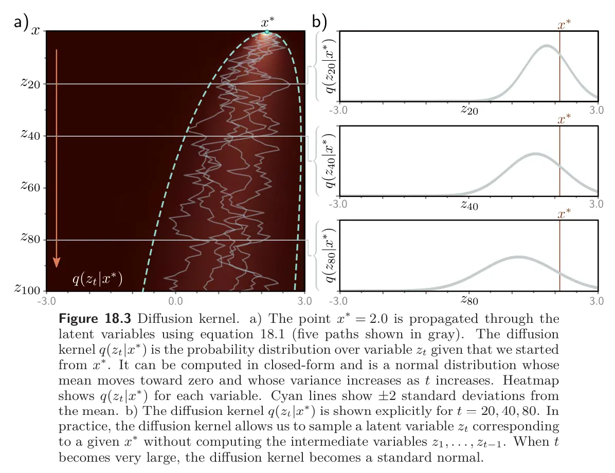
To derive an expression for $q(z_t|x)$, consider the first two steps of the forward process:

$$\begin{array}{rl}{z}_1& =\sqrt{1-{\beta }_1}\cdot x+\sqrt{{\beta }_1}\cdot {ϵ}_1\\ z_2& =\sqrt{1-{\beta }_2}\cdot z_1+\sqrt{{\beta }_2}\cdot {ϵ}_2\end{array}$$

Substituting the first equation into the second, we get:

$$\begin{array}{rl}{z}_2& =\sqrt{1-{\beta }_2}\left(\sqrt{1-{\beta }_1}\cdot x+\sqrt{{\beta }_1}\cdot {ϵ}_1\right)+\sqrt{{\beta }_2}\cdot {ϵ}_2\\ & =\sqrt{1-{\beta }_2}\left(\sqrt{1-{\beta }_1}\cdot x+\sqrt{1-(1-{\beta }_1)}\cdot {ϵ}_1\right)+\sqrt{{\beta }_2}\cdot {ϵ}_2\\ & =\sqrt{(1-{\beta }_2)(1-{\beta }_1)}\cdot x+\sqrt{1-{\beta }_2-(1-{\beta }_2)(1-{\beta }_1)}\cdot {ϵ}_1+\sqrt{{\beta }_2}\cdot {ϵ}_2\end{array}$$

The last two terms are independent samples from mean-zero normal distributions with variances $1-{\beta }_2-(1-{\beta }_2)(1-{\beta }_1)$ and ${\beta }_2$, respectively. The mean of this sum is zero, and its variance is the sum of the component variances (see problem 18.2), so:

$$z_2=\sqrt{(1-{\beta }_2)(1-{\beta }_1)}\cdot x+\sqrt{1-(1-{\beta }_2)(1-{\beta }_1)}\cdot ϵ$$

where $ϵ$ is also a sample from a standard normal distribution.

If we continue this process by substituting this equation into the expression for $z_3$ and so on, we can show that:

$$\begin{array}{rl}{z}_t& =\sqrt{{\alpha }_t}\cdot x+\sqrt{1-{\alpha }_t}\cdot ϵ\\ {\alpha }_t& =\prod _{s=1}^t(1-{\beta }_s)\end{array}$$

We can equivalently write this in probabilistic form:

$$q(z_t|x)={\text{Norm}}_{z_t}[\sqrt{a_t}\cdot x,(1-{\alpha }_t)I]$$

For any starting data point $x$, variable $z_t$ is normally distributed with a known mean and variance. Consequently, if we don’t care about the history of the evolution through the intermediate variables $z_1,\dots ,z_{t-1}$, it is easy to generate samples from $q(z_t|x)$.

Marginal distributions $q(z_t)$

The marginal distribution $q(z_t)$ is the probability of observing a value of $z_t$ given the distribution of possible starting points $x$ and the possible diffusion paths for each starting point.

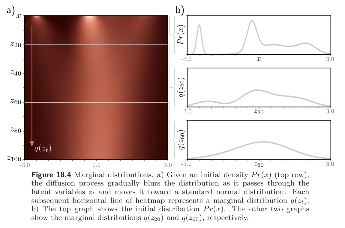
It can be computed by considering the joint distribution $q(x,z_{1\dots t})$ and marginalizing over all the variables except $z_t$:

$$\begin{array}{rl}q(z_t)& =\int \int q(z_{1\dots t},x)d{z}_{1\dots t-1}dx\\ & =\int \int q(z_{1\dots t}|x)Pr(x)d{z}_{1\dots t-1}dx\end{array}$$

where $q(z_{1\dots t}|x)$ was defined above as the joint distribution of all latent variables.

However, since we now have an expression for the diffusion kernel that skips the intervening variables, we can equivalently write:

$$q(z_t)=\int q(z_t|x)Pr(x)dx$$

Hence, if we repeatedly sample from the data distribution $Pr(x)$ and superimpose the diffusion kernel $q(z_t|x)$ on each sample, the result is the marginal distribution $q(z_t)$. However, the marginal distribution cannot be written in closed form because we don’t know the original data distribution $Pr(x)$.

Conditional distribution $q(z_{t-1}|z_t)$

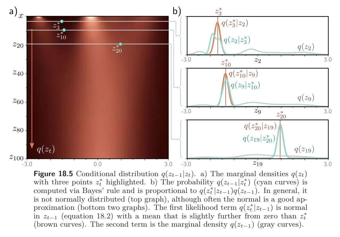
We defined the conditional probability $q(z_t|z_{t-1})$ in the forward process. To reverse this process, we apply Bayes’ Rule:

$$q(z_{t-1}|z_t)=\frac{q(z_t|z_{t-1})q(z_{t-1})}{q(z_t)}$$

This is intractable since we cannot compute the marginal distribution $q(z_{t-1})$.

For simple 1D examples, it’s possible to evaluate $q(z_{t-1}|z_t)$ numerically. In general, their form is complex, but in many cases, they are well-approximated by a normal distribution. This is important because when we build the decoder, we will approximate the reverse process using a normal distribution.

Conditional diffusion distribution $q(z_{t-1}|z_t,x)$

There is one final distribution related to the encoder to consider. We noted above that we could not find the conditional distribution $q(z_{t-1}|z_t)$ because we do not know the marginal distribution $q(z_{t-1})$. However, if we know the starting variable $x$, then we do know the distribution $q(z_{t-1}|x)$ at the time before. This is just the diffusion kernel, and it is normally distributed.

Hence, it is possible to compute the conditional diffusion distribution $q(z_{t-1}|z_t,x)$ in closed form. This distribution is used to train the decoder. It is the distribution over $z_{t-1}$ when we know the current latent variable $z_t$ and the training data example $x$ (which we of course know).

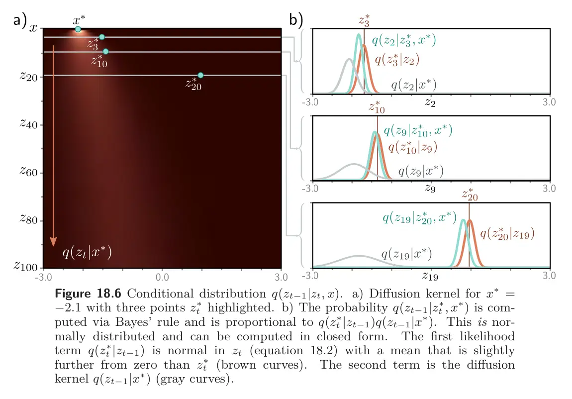
To compute an expression for $q(z_{t-1}|z_t,x)$ we start with Bayes’ rule:

$$\begin{array}{rl}q(z_{t-1}|z_t,x)& =\frac{q(z_t|z_{t-1},x)q(z_{t-1}|x)}{q(z_t|x)}\\ & \propto q(z_t|z_{t-1})q(z_{t-1}|x)\\ & ={\text{Norm}}_{z_t}\left[\sqrt{1-{\beta }_t}\cdot z_{t-1},{\beta }_{t}I\right]{\text{Norm}}_{z_{t-1}}\left[\sqrt{{\alpha }_{t-1}}\cdot x,(1-{\alpha }_{t-1})I\right]\\ & \propto {\text{Norm}}_{z_{t-1}}\left[\frac{1}{\sqrt{1-{\beta }_t}}{z}_t,\frac{{\beta }_t}{1-{\beta }_t}I\right]{\text{Norm}}_{z_{t-1}}[\sqrt{{\alpha }_{t-1}}\cdot x,(1-{\alpha }_{t-1})I]\end{array}$$

• Between the first two lines, we have used the fact that $q(z_t|z_{t-1},x)=q(z_t|z_{t-1})$ because the diffusion process is Markov, and all the information about $z_t$ is captured by $z_{t-1}$.
• Between lines 3 and 4, we use the Gaussian change of variables identity: $${\text{Norm}}_v[Aw,B]\propto {\text{Norm}}_w[(A^T{B}^{-1}A{)}^{-1}{A}^T{B}^{-1}v,(A^T{B}^{-1}A{)}^{-1}]$$ to rewrite the first distribution in terms of $z_{t-1}$.

We then use a second Gaussian identity:

$${\text{Norm}}_w[a,A]\cdot {\text{Norm}}_w[b,B]\propto {\text{Norm}}_w[(A^{-1}+B^{-1}{)}^{-1}(A^{-1}a+B^{-1}b),(A^{-1}+B^{-1}{)}^{-1}]$$

to combine the two normal distributions in $z_{t-1}$, which gives:

$$q(z_{t-1}|z_t,x)={\text{Norm}}_{z_{t-1}}\left[\frac{(1-{\alpha }_{t-1})}{1-{\alpha }_t}\sqrt{1-{\beta }_t}{z}_t+\frac{\sqrt{{\alpha }_{t-1}}{\beta }_t}{1-{\alpha }_t}x,\frac{{\beta }_t(1-{\alpha }_{t-1})}{1-{\alpha }_t}I\right]$$

Note that the constants of proportionality in the equations above must cancel out since the final result is already a correctly normalized probability distribution.