Diffusion Implementation

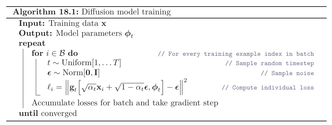
With the reparameterized diffusion loss, we can get straightforward algorithms for both training and sampling diffusion models.

Training algorithm: The training algorithm has the advantages that it is simple to implement. Furthermore, it naturally augments the dataset; we can reuse every original data point $x$, as many times as we want at each time step with different noise instantiations $ϵ$.

Sampling algorithm: The sampling algorithm has the disadvantage that it requires serial processing of many neural networks $g_t[z_t,{\varphi }_t]$ and is hence time-consuming.

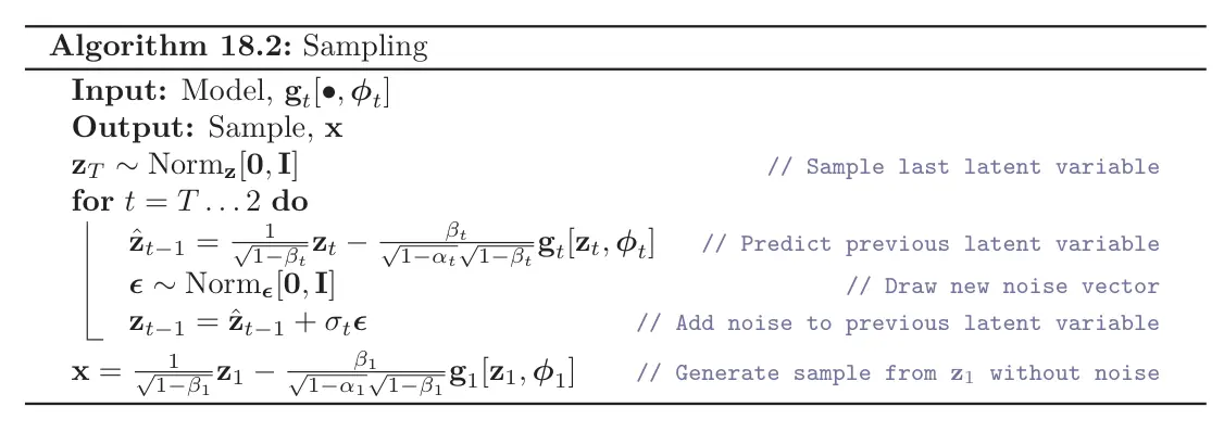
Image Generation

Diffusion models have been very successful in modeling image data. Here, we construct models that can take a noisy image and predict the noise that was added at each step.

The obvious architectural choice for this image-to-image mapping is U-Net; however, there may be a very large number of diffusion steps, and training and storing multiple U-Nets is inefficient. The solution is to train a single U-Net that also takes a predetermined vector representing the time step as input.

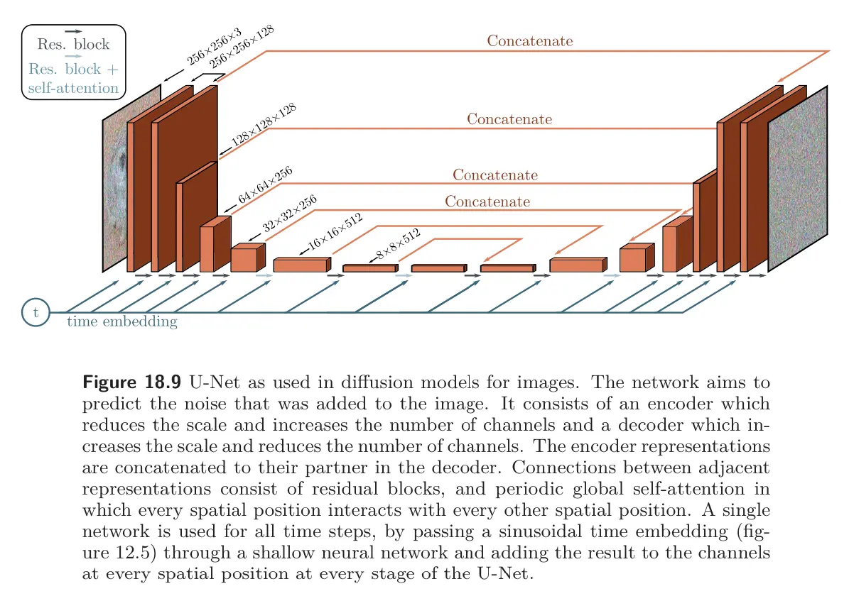
In practice, this is resized to match the number of channels at each stage of the U-Net and used to offset/scale the representation at each spatial position.

A large number of time steps are needed as the conditional probabilities $q(z_{t-1}|z_t)$ become closer to normal when the hyperparameters ${\beta }_t$ are close to zero, matching the form of the decoder distributions $Pr(z_{t-1}|z_t,{\varphi }_t)$. However, this makes sampling slow. We might have to run the U-Net model through $T=1000$ timesteps to generate good images.

Generation speed improvements

The reparameterized diffusion loss requires the diffusion kernel to have the form $q(z_t|x)=\text{ Norm}[\sqrt{\alpha }x,\sqrt{1-{\alpha }_t}]\cdot I$.

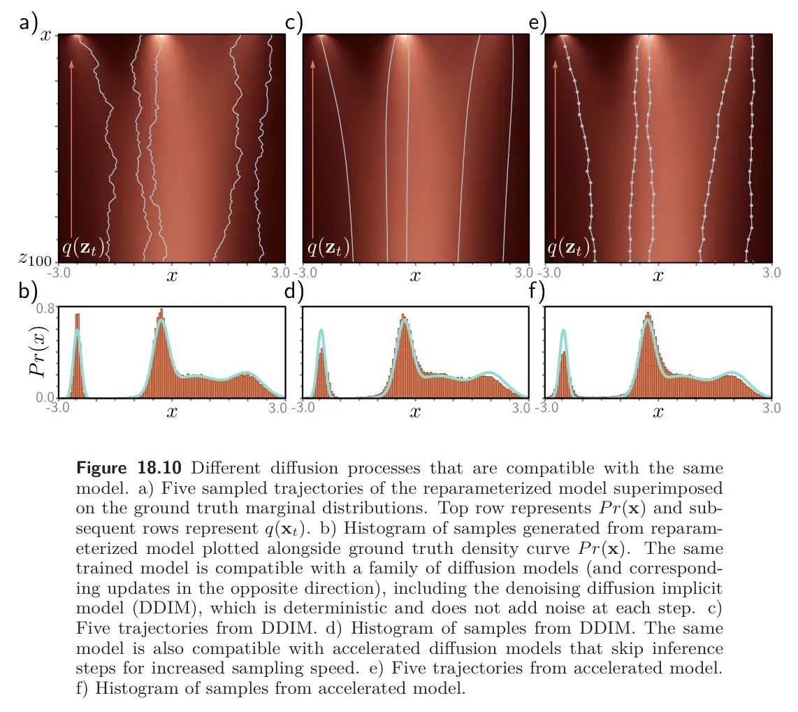
The same loss function will be valid for any forward process with this relation, and there is a family of such compatible processes. These are all optimized by the same loss function but have different rules for the forward process, and different rules for how to use the estimated noise $g[z_t,{\varphi }_t]$ to predict $z_{t-1}$ and $z_t$ in the reverse process.

Among this family are:

• Denoising diffusion implicit models, which are no longer stochastic after the first step from $x$ to $z_1$
• Accelerated sampling models, where the forward process is defined only on a subsequence of time steps.

This allows a reverse process that skips timesteps and hence makes sampling much more efficient. Good samples can be created with 50 time steps when the forward process is no longer stochastic. This is much faster than before but still slower than other generative models.

Conditional generation

If the data has associated labels $c$, these can be exploited to control the generation. Sometimes this can improve generation results in GANs, and we might expect this to be the case in diffusion models as well; it’s easier to denoise an image if you have some information about what the image contains.

One approach to conditional synthesis in diffusion models is classifier guidance. This modifies the denoising update from $z_t$ to $z_{t-1}$ to take into account class information $c$. In practice, this means adding an extra term into the final update step of the sampling algorithm above:

$$z_{t-1}={\hat{z}}_{t-1}+{\sigma }_t^2\frac{\partial \log [Pr(c|z_t)]}{\partial z_t}+{\sigma }_tϵ$$

The new term depends on the gradient of the classifier $Pr(c|z_t)$ that is based on the latent variable $z_t$. This maps features from the downsampling half of the U-Net to the class $c$. Like the U-Net, it is usually shared across all timesteps and takes time as an input. The update from $z_t$ to $z_{t-1}$ now makes the class $c$ more likely.

Classifier-free guidance avoids learning a separate classifier $Pr(c|z_t)$ but instead incorporates class information into the main model $g_t[z_t,{\varphi }_t,c]$. In practice, this usually takes the form of adding an embedding based on $c$ to the layers of the U-Net in a similar way to how the timestep is added (see U-Net diagram above). This model is jointly trained on conditional and unconditional objectives by randomly dropping the class information during training. Hence, it can both generate unconditional or conditional data examples at test time or any weighted combination of the two. This brings a surprising advantage; if the conditioning information is over-weighted, the model tends to produce very high quality but slightly stereotypical examples. This is somewhat analogous to the use of truncation in GANs.

Generation quality improvements

As for other generative models, the highest quality results come from applying a combination of tricks and extensions to the basic model.

First, it’s been noted that it also helps to estimate the variances ${\sigma }_t^2$ of the reverse process as well as the mean. This particularly improves the results when sampling with fewer steps.

Second, it’s possible to modify the noise schedule in the forward process so that ${\beta }_t$ varies at each step, and this can also improve results.

Third, to generate high-resolution images, a cascade of diffusion models can be used. The first creates a low-resolution image (possibly guided by class information). The subsequent diffusion models generate progressively higher-resolution images. They condition on the lower-resolution image by resizing this and appending it to the layers of the constituent U-Net, as well as any other class information.

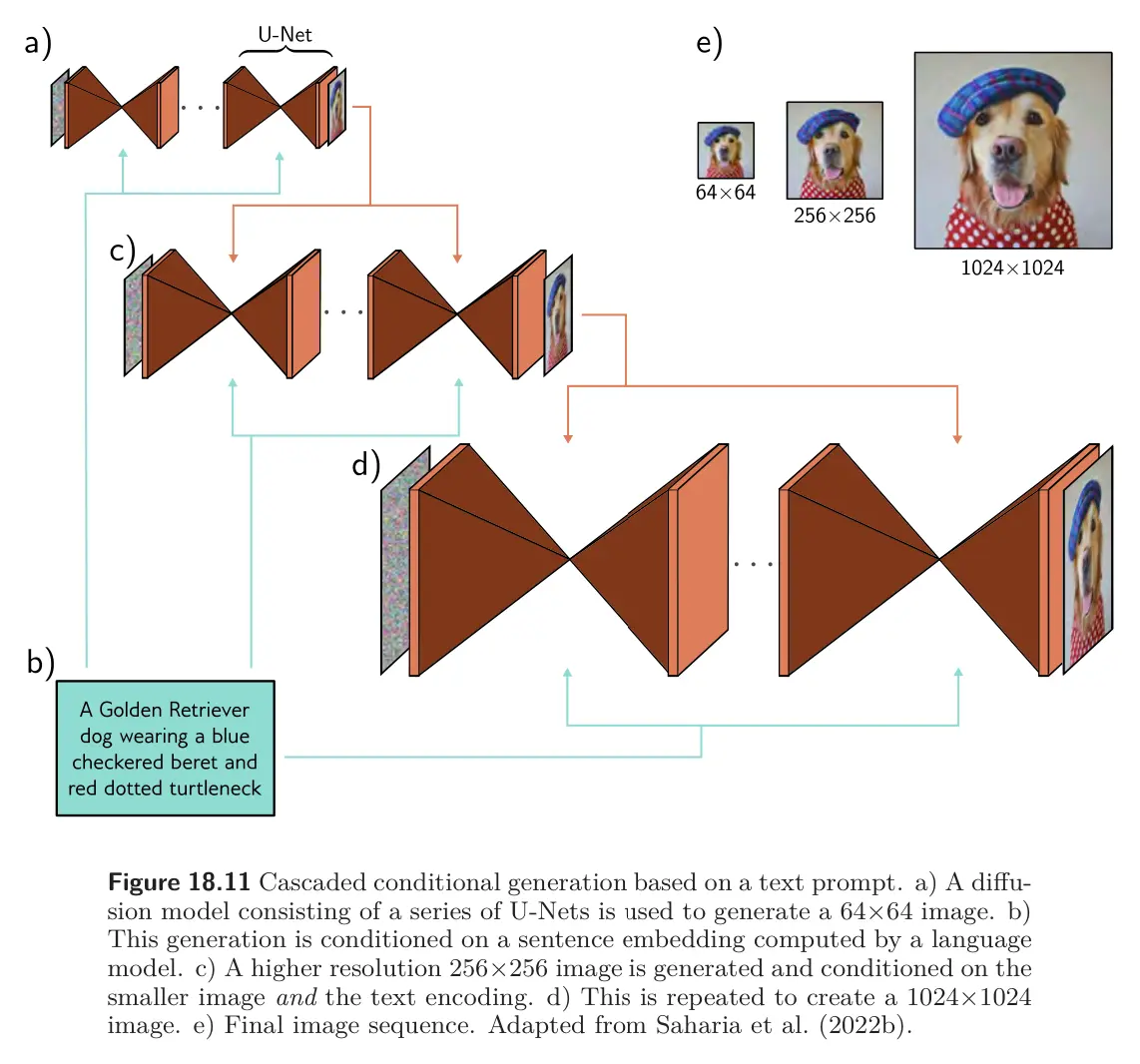
Combining all of these techniques allows for the generation of very high-quality images, with very diverse classes, and following text prompts well. Since diffusion models are stochastic by nature, it is possible to generate multiple images that are conditioned on the same caption.