Generative Adversarial Network

A generative adversarial network or GAN is an unsupervised model that aims to generate new samples that are indistinguishable from a set of training examples.

In a GAN, the main generator network creates samples by mapping random noise to the output data space. If a second discriminator network cannot distinguish between the generated samples and real examples, the samples must be plausible. If the discriminator can tell the difference, this provides a training signal that can be fed back to improve the quality of the samples. The idea is simple, but training GANs can be difficult: the learning algorithm can be unstable, and although GANS may learn to generate realistic samples, this does not mean they learn to generate all possible samples.

GANs just create new samples but do not build a probability over the modeled data, and hence cannot evaluate the probability that a new data point belongs to the same distribution. They have been applied to many types of data, but are most successful in the image domain.

Intuition

Generator: We aim to generate new samples $\{x_j^{\ast }\}$ that are drawn from the same distribution as a set of real training data $\{x_i\}$. A single new new sample $x_j^{\ast }$ is generated by:

1. Choosing a latent variable $z_j$ from a simple base distribution (e.g., a standard normal)
2. Passing this data through a network $x_j^{\ast }=g[z_j,\theta ]$ with parameters $\theta$.

During the learning process, the goal is to find parameters $\theta$ so that the samples $\{x_j^{\ast }\}$ look “similar” to the real data $\{x_i\}$.

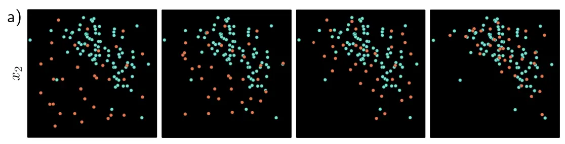
• Generative adversarial models provide a mechanism for generating samples (orange points). As training proceeds (left to right), the loss function encourages these samples to become progressively less distinguishable from real examples (cyan points).

Discriminator: Similarity can be defined in many ways, but the GAN uses the principle that the samples should be statistically indistinguishable. To this end, the discriminator network $f[\bullet ,\varphi ]$ with parameters $\varphi$ is introduced. This aims to classify its input as being a real example or a generated sample. If this is impossible, the generated samples are indistinguishable from the real examples, and we have succeeded. If it is possible, the discriminator provides a signal that can be used to improve the generation process.

Toy example

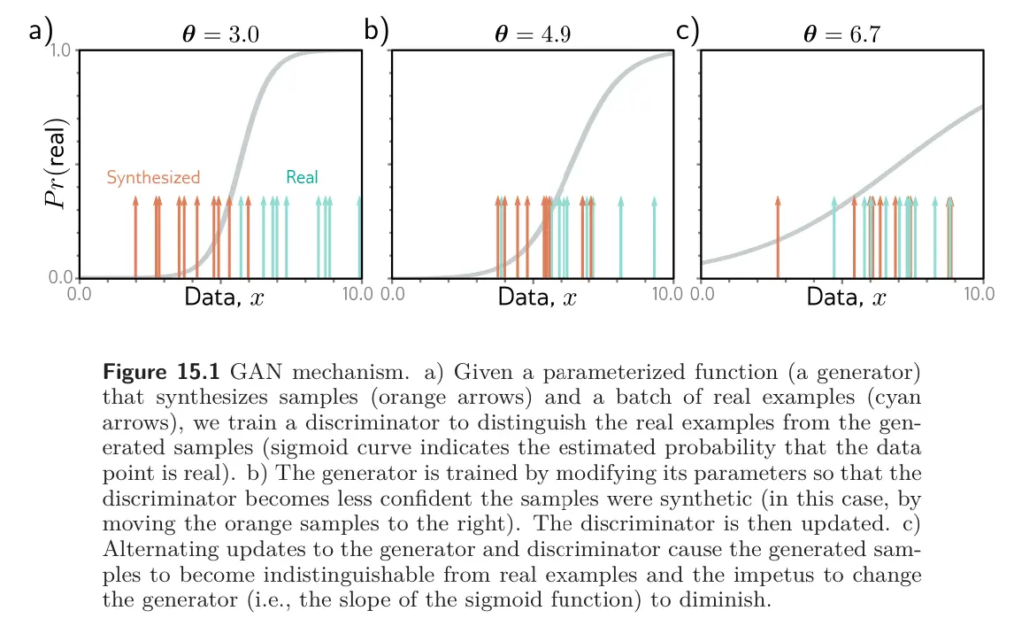
This is illustrated in the figure above. We start with a training set $\{x_i\}$ of real 1D examples. A different batch of these examples $\{x_i{\}}_{i=1}^{10}$ is shown in each panel (cyan arrows). To create a batch of samples $\{x_j^{\ast }\}$, we use the simple generator:

$$x_j^{\ast }=g[z_j,\theta ]=z_j+\theta$$

where latent variables $\{z_j\}$ are drawn from the normal distribution, and the parameter $\theta$ translates the generated samples along the $x$-axis.

At initialization, $\theta =3.0$, and the generated samples (orange arrows) lie to the left of the real examples (cyan arrows). The discriminator is trained to distinguish the generated samples from the real examples (the sigmoid curve indicates the probability that a data point is real). During training, the generator parameters $\theta$ are manipulated to increase the probability that is samples are classified as real. Here, this means increasing $\theta$ so that the samples move rightwards where the sigmoid curve is higher.

We alternate between updating the discriminator and the generator. It gradually becomes harder to classify the data, and the impetus to change $\theta$ becomes weaker (sigmoid becomes flatter). At the end of the process, there is no way to distinguish the two sets of data; the discriminator, which now has 50/50 chance performance, is discarded, and we are left with a generator that makes plausible samples.

Loss function

Let us precisely define the loss function for training GANs.

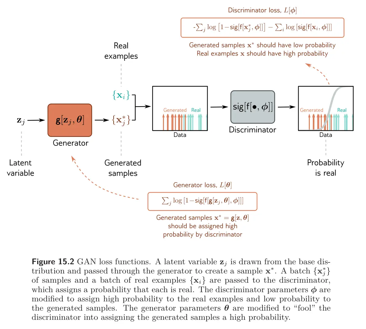
The discriminator $f[x_i,\varphi ]$ takes input $x_i$ and returns a scalar that is higher when it believes the input is real example. This is a binary classification task, so we adapt the binary cross-entropy loss function. Its original form is:

$$\hat{\varphi }=\underset{\varphi }{\mathrm{argmin}}\left[\sum _i-(1-y_i)\log [1-\text{sig}[f[x_i,\varphi ]]]-y_i\log [\text{sig}[f[x_i,\varphi ]]]\right]$$

where $y_i\in \{0,1\}$ is the label. In this case, we assume that the real examples $x$ have label $y=1$ and generated examples $x^{\ast }$ have label $y=0$, which lets us simplify to:

$$\hat{\varphi }=\underset{\varphi }{\mathrm{argmin}}\left[\sum _j-\log [1-\text{sig}[f[x_j^{\ast },\varphi ]]]-\sum _i\log [\text{sig}[f[x_i,\varphi ]]]\right]$$

where $i$ indexes the real examples and $j$ indexes the generated samples.

Now, we can substitute the definition for the generator $x_j^{\ast }=g[z_j,\theta ]$ and note that we must maximize with respect to $\theta$ since we want the generated samples to be misclassified (have low likelihood of being synthetic, or high negative log likelihood). This leads us to:

$$\boxed{\hat{\theta }=\underset{\varphi }{\mathrm{argmax}}\left[\underset{\varphi }{\min }\left[\sum _j-\log [1-\text{sig}[f[g[z_j,\theta ],\varphi ]]]-\sum _i\log [\text{sig}[f[x_i,\varphi ]]]\right]\right]}$$

Training

The GAN loss function is very complex; the discriminator parameters are $\varphi$ are manipulated to minimize the loss function, and the generative parameters are manipulated to maximize the loss function. Thus, GAN training is characterized as a minimax game; the generator tries to find new ways to fool the discriminator, which in turn searches for new ways to distinguish generated samples from real examples. Technically, the solution is a Nash equilibrium – the optimization algorithm searches for a position that is simultaneously a minimum of one function and a maximum of other. If training proceeds as planned, then upon convergence, $g[z,\theta ]$ will be drawn from the same distribution as the data, and $\text{sig}[f[\bullet ,\varphi ]]$ will be at chance (0.5).

To train the GAN, we can divide the above loss function into two loss functions:

$$\begin{array}{rl}L[\varphi ]& =\sum _j-\log [1-\text{sig}[f[g[z_j,\theta ],\varphi ]]]-\sum _i\log [\text{sig}[f[x_i,\varphi ]]]\\ L[\theta ]& =\sum _j\log [1-\text{sig}[f[g[z_j,\theta ],\varphi ]]]\end{array}$$

where we multiplied the second function by $-1$ to convert to a minimization problem and dropped the second term, which has no dependence on $\theta$.

• Minimizing the first loss function trains the discriminator.
• Minimizing the second loss function trains the generator.

At each step, we draw a batch of latent variables $z_j$ from the base distribution and pass these through the generator to create samples $x_j^{\ast }=g[z_j,\theta ]$. Then we choose a batch of real training examples $x_i$. Given the two batches, we can now perform on or more gradient descent steps on each loss function.

dl
GAN
?

• Generator network creates samples by mapping random noise to the output data space.
• Discriminator network tries to classify real examples vs. generated samples.
• Both are trained together in a minimax game where the generator tries to fool the discriminator while the discriminator learns to detect fakes.
• At equilibrium, the generated samples become difficult to distinguish from real data.

+++