Kalman Filter

The Kalman filter is an algorithm that measures the state of a system from measured data. It uses a two-step process: the first step predicts the state of the system, and the second step uses noisy measurements to refine the estimate of system state.

Robot Motion Example

Let’s say we have a robot that has state ${\vec{x}}_k$, which is just a position and velocity:

$${\vec{x}}_k=(\vec{p},\vec{v})$$

State

State is just a list of numbers about the underlying configuration of your system; it could be anything. In our example it’s position and velocity, but it could be data about the amount of fluid in a tank, the temperature of a car engine, the position of a user’s finger on a touchpad, or any number of things you need to keep track of.

Information we have:

• Our robot also has a GPS sensor, which is accurate to about 10 meters, which is good, but not precise enough.
• We also know how the robot moves in general; if it moves in one direction it will, at the next time step it will likely be further along that same direction. However, this is not perfect, as there might be terrain or external factors that result in noise.

Thus, both our sensor and model tell us some information about the state, but only indirectly, and both have some uncertainty. We don’t know what the actual position and velocity are; there are a whole range of possible combinations of position and velocity that might be true, but some of them are more likely than others.

Formulation

The Kalman filter assumes that both position and velocity are random variables that are Gaussian distributed. Each variable has:

• Mean of $\mu$, which is the center of the distribution.
• Variance of $\sigma$, which is the uncertainty.

Covariance

However, it’s important to note that position and velocity could be correlated; the likelihood of observing a particular position depends on what velocity you have:

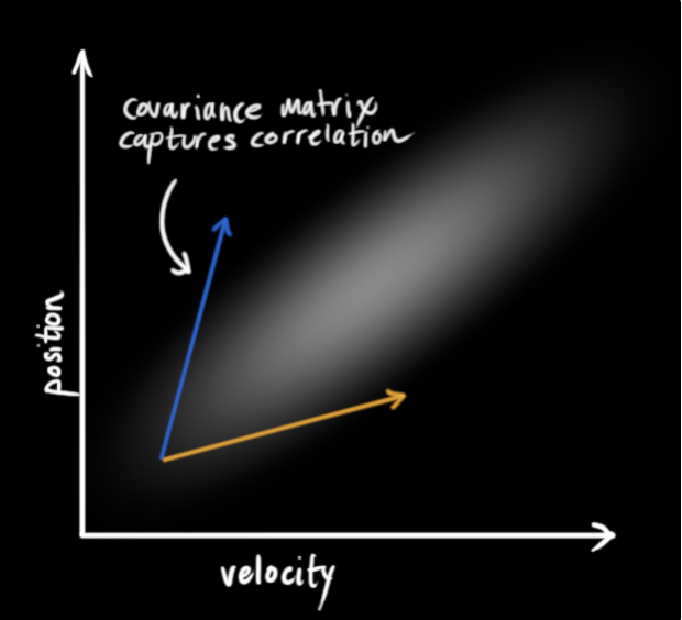
In this case, the correlation between position and velocity is obvious. If our velocity was high, we probably moved farther, so our position will be more distant. This relationship gives us more information about the system; one measurement tells us something about what the others could be.

This correlation is captured by a covariance matrix. Each element ${\sum }_{ij}$ of the matrix is the degree of correlation between the i-th state variable and the j-th state variable.

Prediction Matrix

We’re modeling our knowledge about the state as a Gaussian blob, so we need two pieces of information at time $k$: our best estimate ${\hat{\mathbf{x}}}_k$, and its covariance matrix ${\mathbf{P}}_k$, such that

$$\begin{array}{rl}{\hat{\mathbf{x}}}_k& =\left[\begin{array}{c}\text{position}\\ \text{velocity}\end{array}\right]\\ {\mathbf{P}}_k& =\left[\begin{array}{cc}{\sum }_{pp}& {\sum }_{pv}\\ {\sum }_{vp}& {\sum }_{vv}\end{array}\right]\end{array}$$

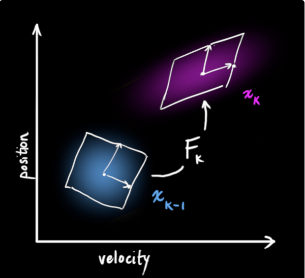
Next, we need to predict the next state at time $k$ based on the current state at $k-1$. This prediction step is done with a prediction matrix ${\mathbf{F}}_k$, which takes every point in our original Gaussian estimate and moves it to a new predicted location.

In our position/velocity example, we can formulate a model based on kinematic laws (assuming constant velocity):

$$\begin{array}{rl}{p}_k& =p_{k-1}+\Delta t{v}_{k-1}\\ v_k& =v_{k-1}\end{array}$$

In matrix form, this is:

$$\begin{array}{rl}{\hat{\mathbf{x}}}_k& =\left[\begin{array}{cc}1& \Delta t\\ 0& 1\end{array}\right]{\hat{\mathbf{x}}}_{k-1}\\ & ={\mathbf{F}}_k{\hat{\mathbf{x}}}_{k-1}\end{array}$$

which gives us our prediction matrix which gives us our next state.

Covariance Matrix

We can update the covariance matrix by observing what happens when we multiply every point in a distribution by a matrix $\mathbf{A}$:

$$\begin{array}{rl}Cov(x)& =\sum \\ Cov(\mathbf{A}x)& =\mathbf{A}\sum {\mathbf{A}}^T\end{array}$$

Thus, our covariance matrix would be updated by:

$${\mathbf{P}}_k={\mathbf{F}}_k{\mathbf{P}}_{k-1}{\mathbf{F}}_k^T$$

This is also called the process noise covariance matrix.

Control Matrix & Control Vector

If we know any additional information about the world, we can stuff it into a vector called ${\vec{\mathbf{u}}}_k$ and add it to our prediction as a correction.

Let’s say we know the expected acceleration 𝑎 due to the throttle setting or control commands. From basic kinematics we get:

$$\begin{array}{rl}{p}_k& =p_{k-1}+\Delta t{v}_{k-1}+\frac{1}{2}a\Delta t^2\\ v_k& =v_{k-1}+a\Delta t\end{array}$$

In matrix form:

$$\begin{array}{rl}{\hat{\mathbf{x}}}_k& ={\mathbf{F}}_k{\hat{\mathbf{x}}}_{k-1}+\left[\begin{array}{c}\frac{\Delta t^2}{2}\\ \Delta t\end{array}\right]a\\ & ={\mathbf{F}}_k{\hat{\mathbf{x}}}_{k-1}+{\mathbf{B}}_k{\vec{\mathbf{u}}}_k\end{array}$$

Here, ${\mathbf{B}}_k$ is the control matrix and ${\vec{\mathbf{u}}}_k$ is the control vector. For very simple systems with no external influence, we can omit these.

Uncertainty

We can model the uncertainty associated with the “world” (i.e. things we aren’t keeping track of or can’t control) by adding some new uncertainty after every prediction step. Every state in our original estimate could have moved to a range of states; each point in ${\hat{\mathbf{x}}}_{k-1}$ is moved to somewhere inside a Gaussian blob with covariance ${\mathbf{Q}}_k$. Another way to say this is that we are treating the untracked influences as noise with covariance ${\mathbf{Q}}_k$ – this is called the process noise covariance matrix.

We get the expanded covariance by simply adding ${\mathbf{Q}}_k$, giving our complete expression for the prediction step.

Prediction Step

$$\begin{array}{rl}& \\ {\hat{\mathbf{x}}}_k& ={\mathbf{F}}_k{\hat{\mathbf{x}}}_{k-1}+{\mathbf{B}}_k{\vec{\mathbf{u}}}_k\\ {\mathbf{P}}_k& ={\mathbf{F}}_k{\mathbf{P}}_{k-1}{\mathbf{F}}_k^T+{\mathbf{Q}}_k\end{array}$$

As such, the new best estimate is is a prediction made from previous best estimate, plus a correction for known external influences. The new uncertainty is predicted from the old uncertainty, with some additional uncertainty from the environment.

Measurement

We might have several sensors which give us information about the state of our system. These give indirect readings; based on the state, the sensors have some transfer function/mapping to their measurement:

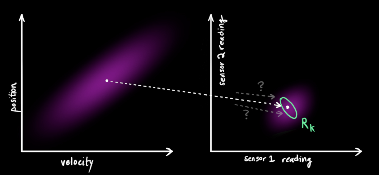
This transfer function can for the sensors can be modeled with a matrix, ${\mathbf{H}}_k$; it takes a predicted state vector ${\hat{\mathbf{x}}}_k$ and turns it into a predicted measurement vector (what the sensor reading should be). This sensor reading distribution is given by:

$$\begin{array}{r}{\vec{\mu }}_{\text{expected}}={\mathbf{H}}_k{\hat{\mathbf{x}}}_k\\ {\Sigma }_{\text{expected}}={\mathbf{H}}_k{\mathbf{P}}_k{\mathbf{H}}_k^T\end{array}$$

We also need to deal with sensor noise; every very state in our original estimate might result in a range of sensor readings. The covariance of this uncertainty (sensor noise) is called $\mathbf{R}$ – this is called the measurement noise covariance matrix.

The distribution has a mean equal to the reading we observed, which we’ll call ${\vec{\mathbf{z}}}_k$.

Combining Gaussians

Now we have two Gaussian blobs: one for our prediction, and one surrounding the actual sensor reading we got, which we must reconcile.

For any possible reading $(z_1,z_2)$, we have two associated probabilities:

1. The probability that our sensor reading ${\vec{\mathbf{z}}}_k$ is a mis-measurement of $(z_1,z_2)$
2. The probability that our previous estimate thinks $(z_1,z_2)$ is the reading we should see.

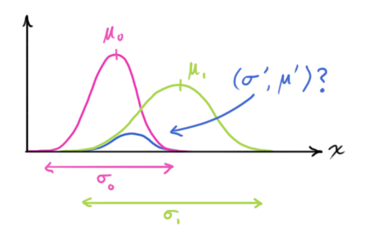
If we two probabilities and we want to know the chance that both are true, we just multiply them together. We’re left with the overlap, the region where both blobs are likely. The mean of this distribution is the state for which both estimates are most likely, and is therefore the best guess of the true state given all the information we have.

A distribution found by multiplying two distributions together is given by:

$$\begin{array}{rl}\mathbf{k}& =\frac{{\sigma }_0^2}{{\sigma }_0^2+{\sigma }_1^2}\\ {\mu }^{\prime }& ={\mu }_0+\mathbf{k}({\mu }_1-{\mu }_0)\\ {\sigma }^{\prime 2}& ={\sigma }_0^2-\mathbf{k}{\sigma }_0^2\end{array}$$

The matrix version of this is:

$$\begin{array}{rl}\mathbf{K}& ={\Sigma }_0({\Sigma }_0+{\Sigma }_1{)}^{-1}\\ {\vec{\mu }}^{\prime }& ={\vec{\mu }}_0+\mathbf{K}({\vec{\mu }}_1-{\vec{\mu }}_0)\\ {\Sigma }^{\prime }& ={\Sigma }_0-\mathbf{K}{\Sigma }_0\end{array}$$

$\mathbf{K}$ is a matrix called the Kalman gain, which essentially represents the weight given to the difference between the actual measurement and the predicted state.

• If the Kalman gain is high, the filter places more trust in the latest measurements.
• Conversely, a low Kalman gain indicates more confidence in the model predictions.

Update Step

We have two distributions:

• Prediction: $({\mu }_0,{\Sigma }_0)=({\mathbf{H}}_k{\hat{\mathbf{x}}}_{\mathbf{k}},{\mathbf{H}}_{\mathbf{k}}{\mathbf{P}}_{\mathbf{k}}{{\mathbf{H}}_{\mathbf{k}}}^{\mathbf{T}})$
• Measurement: $({\mu }_1,{\Sigma }_1)=({\vec{\mathbf{z}}}_k,{\mathbf{R}}_k)$

Finding the overlap between these:

$$\begin{array}{rl}{\mathbf{H}}_k{\hat{\mathbf{x}}}_k^{\prime }& ={\mathbf{H}}_{\mathbf{k}}{\hat{\mathbf{x}}}_k+\mathbf{K}({\vec{\mathbf{z}}}_k-{\mathbf{H}}_k{\hat{\mathbf{x}}}_k)\\ {\mathbf{H}}_k{\mathbf{P}}_k^{\prime }{\mathbf{H}}_k^T& ={\mathbf{H}}_k{\mathbf{P}}_k{\mathbf{H}}_k^T-\mathbf{K}{\mathbf{H}}_k{\mathbf{P}}_k{\mathbf{H}}_k^T\end{array}$$

The Kalman gain is:

$$\mathbf{K}={\mathbf{H}}_k{\mathbf{P}}_k{\mathbf{H}}_k^T({\mathbf{H}}_k{\mathbf{P}}_k{\mathbf{H}}_k^T+{\mathbf{R}}_k{)}^{-1}$$

We can remove ${\mathbf{H}}_k$ from every term:

$$\begin{array}{rl}{\hat{\mathbf{x}}}_k^{\prime }& ={\hat{\mathbf{x}}}_k+{\mathbf{K}}^{\prime }({\vec{\mathbf{z}}}_k-{\mathbf{H}}_k{\hat{\mathbf{x}}}_k)\\ {\mathbf{P}}_k^{\prime }& ={\mathbf{P}}_k-{\mathbf{K}}^{\prime }{\mathbf{H}}_k{\mathbf{P}}_k\\ {\mathbf{K}}_k^{\prime }& ={\mathbf{P}}_k{\mathbf{H}}_k^T({\mathbf{H}}_k{\mathbf{P}}_k{\mathbf{H}}_k^T+{\mathbf{R}}_k{)}^{-1}\end{array}$$

That’s it! Our new best estimate is ${\hat{\mathbf{x}}}_k^{\prime }$, and we can go on and feed it (along with ${\mathbf{P}}_k^{\prime }$) back in, to predict or update as many times as we like.