Track-to-Track Fusion

Tracking Architectures

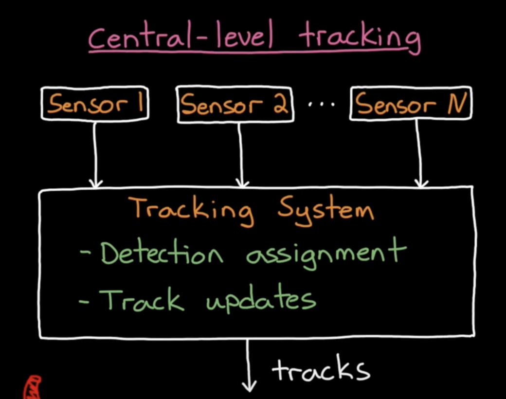
Central-level Tracking

The standard “central-level” tracking algorithm operates as such:

1. Sensor detections fed into a tracking algorithm that assigns the detections to tracks
2. Update the state and covariance of the tracked object

Here, all sensor-data is fused at the same level and within the same tracker. As long as sensor measurements feed into a central tracker, no matter what it’s tracking, we can think of it as a central-level tracker.

Track-level Fusion with Sensor-level Tracking

The idea here is that one or more sensors feed into a tracker, just like the above central-level architecture. But now, we have several of these trackers, each fusing together its own set of sensors and producing its own track estimate. We then have a track-level fuser for track assignment and central track updating.

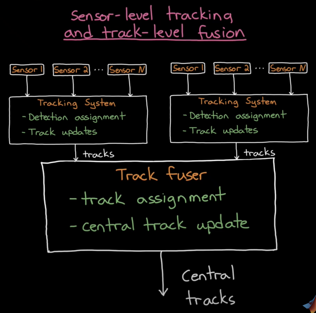
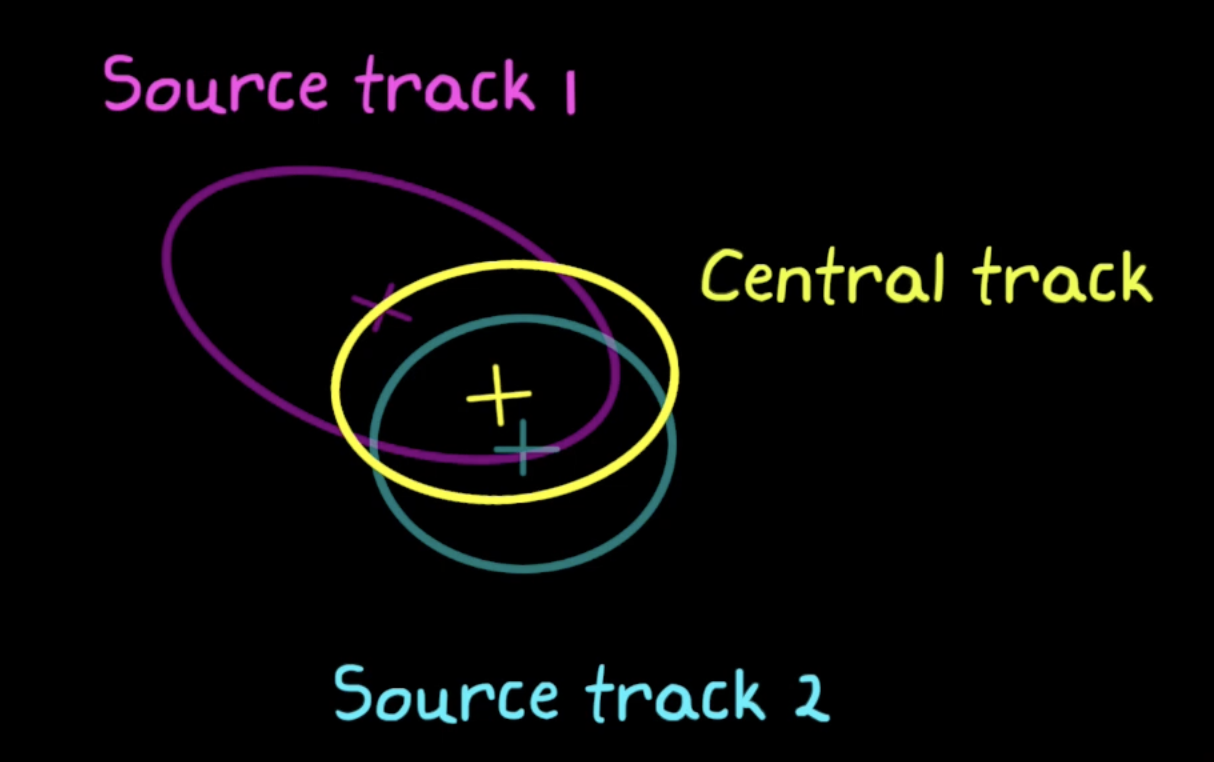
For example, two sensor-level tracker might produce two probability distributions; it’s then up to the track fuser to determine if these two tracks are two different objects, or associate them as the same object.

Benefits

Track-to-track fusion has several benefits:

• Access to data: We can use track-level fusion without access to raw data; for example, many sensors have built-in tracking algorithm, which return a state matrix with $[\text{position, velocity, orientation, shape}]$ and a set of covariance matrices indicating how much confidence there is in each state.
• Bandwidth: If we have limited bandwidth, track-level fusion allows us to send less information to the main computer running the track-level fuser.
• Compute: Similar to bandwidth, using track-level fusion allows us to distribute our compute across sensors, so that our central tracker doesn’t have to run a massive central-level algorithm.
• Specialization: Our sensor-level trackers can be specialized to their specific sensor type. In a tracker we have to set up motion models and sensor models, and associate detections with objects and tracks. We have to tune this to a particular set of hardware; doing sensor-level tracking makes this easier and more modular. Instead of a single large-scale tracking algorithm, we have a bunch of smaller ones, making it easier to tune and test.

Challenges

Track-to-track fusion suffers from three main challenges:

• Correlated noise: If the tracks that we are fusing together are correlated in some way, we can’t just multiply their probabilities like we can in a standard Kalman Filter. For example, if two trackers use the same process model, fusing their outputs together does not improve confidence since we’re not getting any more information.
  • The problem it’s hard to tell when two trackers are correlated. There are some solutions such as Covariance Intersection.
• Reduced accuracy: Track-to-track fusion is a “late” fusion scheme, as we are fusing tracks produced by sensor-level trackers and not raw data. Thus, we may be losing information before the track-level fusion stage.
• Rumor propagation: When fusing sensors with different ranges or fields of view, it can be nice for Car A that can’t see some a pedestrian to have it in its tracks because Car B that can see it propagated it. However, it’s important that when the pedestrian is no longer detected by Sensor B, this change is reflected in Sensor A’s world model, and that Sensor A does not erroneously tell Sensor B that this object still exists. Otherwise, both will still think that the pedestrian is still there.