Parameter Initialization

How do we initialize parameters before training?

To see why this is crucial, consider that during the forward pass, each set of pre-activations ${\mathbf{f}}_k$ is computed as:

$$\begin{array}{rl}{\mathbf{f}}_k& ={\beta }_k+{\mathbf{\Omega }}_k{\mathbf{h}}_k\\ & ={\beta }_k+{\mathbf{\Omega }}_{\mathbf{k}}\mathbf{a}[{\mathbf{f}}_{k-1}]\end{array}$$

where $\mathbf{a}[\bullet ]$ applies the ReLU function and ${\Omega }_k$ and ${\beta }_k$ are the weights and biases.

Imagine that we initialize all the biases to zero and elements of ${\mathbf{\Omega }}_k$ according to a normal distribution with mean zero and variance ${\sigma }^2$. Consider two scenarios:

1. If the variance ${\sigma }^2$ is very small, then each element of ${\beta }_k+{\mathbf{\Omega }}_k{\mathbf{h}}_k$ will be a weighted sum of ${\mathbf{h}}_k$ where the weights are very small; the result will likely have a smaller magnitude than the input. In addition, ReLU clips values less than zero, so the range of ${\mathbf{h}}_k$ will be half that of ${\mathbf{f}}_{k-1}$. Consequently, the magnitudes of the pre-activations at the hidden layers will get smaller and smaller as we progress throughout the network.
2. If the variance ${\sigma }^2$ is very large, then each element of ${\beta }_k+{\mathbf{\Omega }}_k{\mathbf{h}}_k$ will be a weighted sum of ${\mathbf{h}}_k$ where the weights are very large; the result is likely to have much larger magnitude than the input. ReLU function halves the range of the inputs, but if ${\sigma }^2$ is large enough, the magnitudes of the pre-activations will still get larger as we progress through the network.

In these two situations, the values at the pre-activations can become so small or so large that they cannot be represented with finite precision floating point arithmetic. Even if the forward pass is tractable, the same logic applies to the backward pass. Each gradient update consists of multiplying by ${\mathbf{\Omega }}^T$. If the values of $\Omega$ are not initialized sensibly, then the gradient magnitudes may decrease or increase uncontrollably during the backward pass. These cases are known as the exploding gradient gradient problem, respectively. In the former case, updates to the model become vanishingly small. In the latter case, they become unstable.

Initialization for Forward Pass

Consider the computation between pre-activations $\mathbf{f}$ and ${\mathbf{f}}^{\prime }$ with dimensions $D_h$ and $D_{h^{\prime }}$, respectively:

$$\begin{array}{rl}\mathbf{h}& =\mathbf{a}[\mathbf{f}]\\ {\mathbf{f}}^{\prime }& =\beta +\mathbf{\Omega h}\end{array}$$

where $\mathbf{h}$ represents the activations, $\mathbf{\Omega }$ and $\beta$ represent the weights and biases, and $\mathbf{a}[\bullet ]$ is the activation function.

Purpose

Our aim here is to derive an expression for the variance of the output pre-activations ${\mathbf{f}}^{\prime }$ as a function of the variance of the the input layer $\mathbf{f}$. Then, we can use this to reason about how we should initialize so that the variance stays stable.

Assume the pre-activations $f_j$ in the input layer $\mathbf{f}$ have variance ${\sigma }_f^2$. The biases ${\beta }_i$ are initialized to zero, and the weights ${\Omega }_{ij}$ are initialized as normally distributed with mean zero and variance ${\sigma }_{\Omega }^2$.

Now we derive expressions for the mean of the pre-activations ${\mathbf{f}}^{\prime }$ in the subsequent layer.

The mean for each row $f_i^{\prime }$ of the pre-activation $\mathbf{f}$:

$$\begin{array}{rl}\mathbb{E}[f_i^{\prime }]& =\mathbb{E}\left[{\beta }_i+\sum _{j=1}^{D_h}{\Omega }_{ij}{h}_j\right]\\ & =\mathbb{E}[{\beta }_i]+\sum _{j=1}^{D_h}\mathbb{E}[{\Omega }_{ij}{h}_j]\\ & =\mathbb{E}[{\beta }_i]+\sum _{j=1}^{D_h}\mathbb{E}[{\Omega }_{ij}]\mathbb{E}[h_j]\\ & =0+\sum _{j=1}^{D_h}0\cdot \mathbb{E}[j_j]\\ & =0\end{array}$$

• This assumes that the distribution over the hidden units $h_j$ and the network weights ${\Omega }_{ij}$ are independent between the second and third lines.

Using this result, we see that the variance, ${\sigma }_f^2$ of the pre-activations $f_i^{\prime }$ is:

$$\begin{array}{rl}{\sigma }_{f^{\prime }}^2& =\mathbb{E}[f_i^{\prime 2}]-\mathbb{E}[f_i{]}^2\\ & =\mathbb{E}\left[{\left({\beta }_i+\sum _{j=1}^{D_h}{\Omega }_{ij}{h}_j\right)}^2\right]-0\\ & =\mathbb{E}\left[{\left(\sum _{j=1}^{D_h}{\Omega }_{ij}{h}_j\right)}^2\right]\\ & =\sum _{j=1}^{D_h}\mathbb{E}[{\Omega }_{ij}^2]\mathbb{E}[h_j^2]\\ & =\sum _{j=1}^{D_h}{\sigma }_{\Omega }^2\mathbb{E}[h_j^2]\\ & ={\sigma }_{\Omega }^2\sum _{j=1}^{D_h}\mathbb{E}[h_j^2]\end{array}$$

where we have used the variance identity ${\sigma }^2=\mathbb{E}[(z-\mathbb{E}[z]{)}^2]=\mathbb{E}[z^2]-\mathbb{E}[z{]}^2$. We’ve also assumed again that the distribution of the weights ${\Omega }_{ij}$ and the hidden units $h_j$ are independent between lines 3 and 4.

Assuming that the distribution of pre-activations $f_j$ at the previous layer is symmetric about zero, half of these pre-activations are clipped by the ReLU function, and the second moment $\mathbb{E}[h_j^2]$ will be half of ${\sigma }_f^2$, the variance of $f_j$:

$${\sigma }_{f_i^{\prime }}^2={\sigma }_{\Omega }^2\sum _{j=1}^{D_h}\frac{{\sigma }_f^2}{2}=\frac{1}{2}{D}_h{\sigma }_{\Omega }^2{\sigma }_f^2$$

This implies that if we want the variance ${\sigma }_{f^{\prime }}^2$ of the subsequent pre-activations ${\mathbf{f}}^{\prime }$ to be the same as the variance ${\sigma }_f^2$ of the original pre-activations $\mathbf{f}$ during the forward pass, we should set

$${\sigma }_{\Omega }^2=\frac{2}{D_h}$$

where $D_h$ is the dimension of the original layer to which the weights were applied. This is known as He initialization.

Initialization for backward pass

A similar argument establishes how the variance of the gradients $\partial \ell /\partial f_k$ changes during the backward pass. During the backward pass, we multiply by the transpose ${\mathbf{\Omega }}^T$ of the weight matrix, so the equivalent expression becomes:

$${\sigma }_{\Omega }^2=\frac{2}{D_h^{\prime }}$$

where $D_h^{\prime }$ is the dimension of the layer that the weights feed into.

Initialization for both forward & backward

If the weight matrix $\mathbf{\Omega }$ is not square (there are different numbers of hidden units in the two adjacent layers, so $D_h$ and $D_h^{\prime }$ differ), then it is not possible to choose the variance to satisfy both ${\sigma }_{\Omega }^2=\frac{2}{D_h}$ and ${\sigma }_{\Omega }^2=\frac{2}{D_h^{\prime }}$ simultaneously.

One possible compromise is to use the mean $(D_h+D_h^{\prime })/2$ as a proxy for the number of terms, which gives:

$${\sigma }_{\Omega }^2=\frac{4}{D_h+D_h^{\prime }}$$

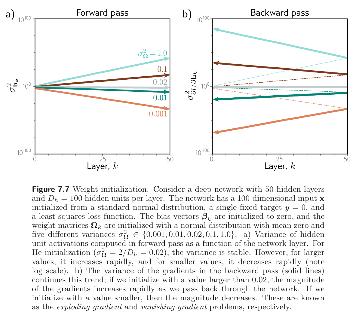
The figure below shows empirically that both the variance of the hidden units in the forward pass and the variance of the gradients in the backward pass remain stable when the parameters are initialized appropriately.