Simple Static State Estimation Example

Weighing Gold Example

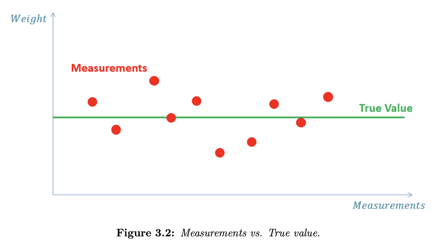
In this example, we estimate the state of a static system. A static system is a system that doesn’t change its state over a reasonable period. Here, we we estimate the weight of the gold bar. We have unbiased scales (the measurements don’t have a systematic error), but the measurements do include random noise.

• System: Gold bar
• System state: Weight of gold bar
• Model: The dynamic model of the system is constant since we assume that the weight doesn’t change over short periods

To estimate the system state (i.e., the weight value), we can make multiple measurements and average them.

At the time $n$, an estimate ${\hat{x}}_{n,n}$ would be the average of all previous measurements:

$${\hat{x}}_{n,n}=\frac{1}{n}(z_1+z_2+\cdots +z_{n-1},z_n)=\frac{1}{n}\sum _{i=1}^n(z_i)$$

• $x$ is the true value of the weight
• $z_n$ is the measured value of the weight at time $n$
• ${\hat{x}}_{n,n}$ is the estimate of $x$ at time $n$ (the estimate is made after taking the measurement $z_n$)
• ${\hat{x}}_{n+1,n}$ is the estimate of the future state ($n+1$) of $x$. The estimate is made at the time $n$. In other words, ${\hat{x}}_{n+1,n}$ is a predicted state or extrapolated state.
• ${\hat{x}}_{n-1,n-1}$ is the estimate of $x$ at time $n-1$ (the estimate is made after taking the measurement $z_{n-1}$).
• ${\hat{x}}_{n,n-1}$ is a prior prediction – the estimate of the state at time $n$. The prediction is made at the time $n-1$.
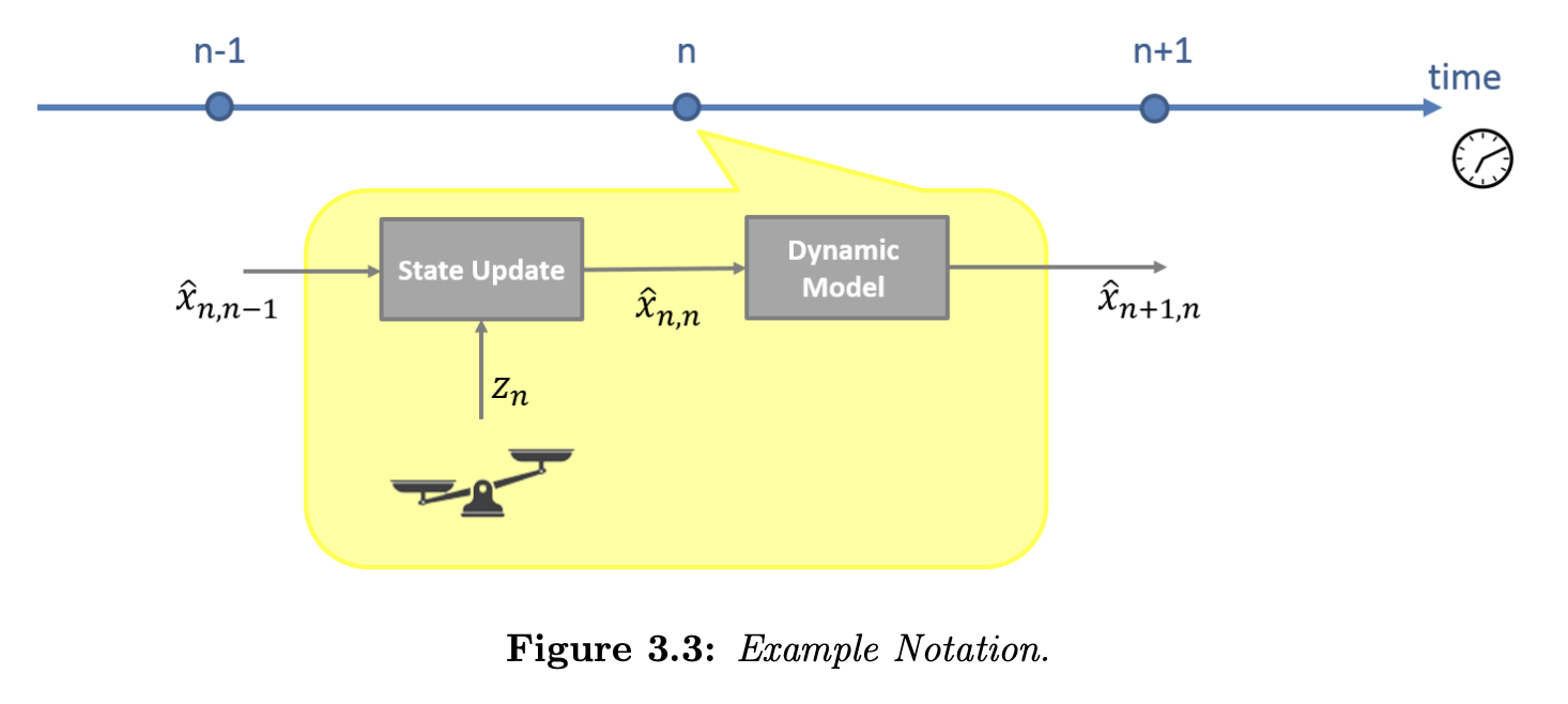
  • Basically, the first subscript is the time we are making the estimate for. The second subscript is the time at which the estimate is made.

The dynamic model in this example is static/constant since the weight of gold doesn’t change over time, therefore ${\hat{x}}_{n+1,n}={\hat{x}}_{n,n}$.

Although our previous equation for ${\hat{x}}_{n,n}$ is mathematically correct, it is not practical for implementation. In order to estimate ${\hat{x}}_{n,n}$, we need to remember all historical measurements; therefore, we need a large memory. We also need to recalculate the average repeatedly if we want to update the estimated value after every new measurement.

It would be more practical to only keep the last estimate, (${\hat{x}}_{n-1,n-1}$) and update it after every new measurement. The following figure exemplifies the required algorithm:

• Estimate the current state based on the measurement and prior prediction.
• Predict the next state based on the current state estimate using the Dynamic Model.

We can modify the averaging equation for our needs using a small mathematical trick.

First, we have the average formula (sum of $n$ measurements divided by $n$):

$${\hat{x}}_{n,n}=\frac{1}{n}\sum _{i=1}^n{z}_i$$

We can re-arrange this as the sum of $n-1$ measurements plus the last measurement divided by $n$:

$${\hat{x}}_{n,n}=\frac{1}{n}\left(\sum _{i=1}^{n-1}(z_i)+z_n\right)$$

Expanding:

$${\hat{x}}_{n,n}=\frac{1}{n}\sum _{i=1}^{n-1}(z_i)+\frac{1}{n}{z}_n$$

Multiplying the first term by $\frac{n-1}{n-1}$:

$${\hat{x}}_{n,n}=\frac{1}{n}\frac{n-1}{n-1}\sum _{i=1}^{n-1}(z_i)+\frac{1}{n}{z}_n$$

Re-order:

$${\hat{x}}_{n,n}=\frac{n-1}{n}\underset{\text{Prior estimate }}{\underbrace{\frac{1}{n-1}\sum _{i=1}^{n-1}(z_i)}}+\frac{1}{n}{z}_n$$

Re-writing the sum:

$${\hat{x}}_{n,n}=\frac{n-1}{n}{\hat{x}}_{n-1,n-1}+\frac{1}{n}{z}_n$$

Distributing the term $\frac{n-1}{n}$:

$${\hat{x}}_{n,n}=\cancel{\frac{n}{n}}{\hat{x}}_{n-1,n-1}-\frac{1}{n}{\hat{x}}_{n-1,n-1}+\frac{1}{n}{z}_n$$

Re-ordering:

$$\boxed{{\hat{x}}_{n,n}={\hat{x}}_{n-1,n-1}+\frac{1}{n}(z_n-{\hat{x}}_{n-1,n-1})}$$

Recall that ${\hat{x}}_{n-1,n-1}$ is the estimated state of $x$ at time $n-1$ based on the measurement at the time $n-1$.

Let’s find ${\hat{x}}_{n,n-1}$ (the predicted state of $x$ at the time $n$), based on ${\hat{x}}_{n-1,n-1}$ (the estimation at the time $n-1$). In other words, we would like to extrapolate ${\hat{x}}_{n-1,n-1}$ to the time $n$. Since the dynamic model in this example is static, the predicted state of $x$ equals the estimated state of $x$ with:

$${\hat{x}}_{n,n-1}={\hat{x}}_{n-1,n-1}$$

Based on the above, we can write the State Update Equation:

$${\hat{x}}_{n,n}={\hat{x}}_{n,n-1}+\frac{1}{n}(z_n-{\hat{x}}_{n,n-1})$$

The State Update Equation is one of the five Kalman filter equations. It means the following:

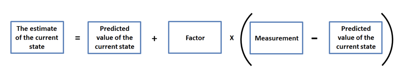
The factor $1/n$ is specific to our example. This is called the Kalman Gain. It is denoted by $K_n$. The subscript $n$ indicates that the Kalman Gain can change with every iteration.

Before we get into the Kalman Filter in depth, we will use the Greek letter ${\alpha }_n$ instead of $K_n$:

$${\hat{x}}_{n,n}={\hat{x}}_{n,n-1}+{\alpha }_n(z_n-{\hat{x}}_{n,n-1})$$

The term $(z_n-{\hat{x}}_{n,n-1})$ is called the measurement residual or innovation – this is the difference between the actual measured state and the state previously predicted based on past information. The innovation contains past information.

In this example, $1/n$ decreases as $n$ increases. In the beginning, we don’t have enough information about the current state; thus, the first estimation is based on the first measurement $\frac{1}{n}{|}_{n=1}=1$ . As we continue, each successive measurement has less weight in the estimation process, since $1/n$ decreases. At some point, the contribution of the new measurements will become negligible.

Let’s continue with the example. Before we make the first measurement, we can guess (or rough estimate) the gold bar weight simply by reading the stamp on the gold bar. It is called the initial guess, and it is our first estimate. The Kalman Filter requires the initial guess as a preset, which can be very rough.

Numerical Example

Iteration 0

Initialization: Our initial guess of the gold bar weight is 1000 grams. The initial guess is used only once for the filter initiation. Thus, it won’t be required for successive iterations.

$${\hat{x}}_{0,0}=1000g$$

Prediction: The weight of the gold bar is not supposed to change. Therefore, the dynamic model of the system is static. Our next state estimate (prediction) equals the initialization:

$${\hat{x}}_{1,0}=1000g$$

Iteration 1

Making the weight measurement with the scales:

$$z_1=996g$$

Calculating the gain. In our example, ${\alpha }_n=\frac{1}{n}$, so we have

$${\alpha }_1=\frac{1}{1}=1$$

Calculating the current estimate using the state update equation:

$${\hat{x}}_{1,1}={\hat{x}}_{1,0}+{\alpha }_1(z_1-{\hat{x}}_{1,0})=1000+1(996-1000)=996g$$

The dynamic model of the system is static; thus our next state estimate (prediction) is the same as the current state estimate:

$${\hat{x}}_{2,1}={\hat{x}}_{1,1}=996g$$

Iteration 2

After a unit time delay, , the predicted estimate from the previous iteration becomes the prior estimate in the current iteration:

$${\hat{x}}_{2,1}=996g$$

Making a second weight measurement:

$$z_2=994g$$

Calculating the gain:

$$a_2=\frac{1}{2}$$

Calculating the current estimate:

$$\begin{array}{rl}{\hat{x}}_{2,2}& ={\hat{x}}_{2,1}+\alpha (z_2-{\hat{x}}_{2,1})\\ & =996+\frac{1}{2}(994-996)=995g\end{array}$$

Calculating the prediction:

$${\hat{x}}_{3,2}={\hat{x}}_{2,2}=995g$$

Iteration 3

$$\begin{array}{rl}{z}_3& =1021g\\ a_3& =\frac{1}{3}\\ {\hat{x}}_{3,3}& =995+\frac{1}{3}(1021-995)=1003.67g\\ {\hat{x}}_{4,3}& ={\hat{x}}_{3,3}=1003.67g\end{array}$$

Iteration 4

$$\begin{array}{rl}{z}_4& =1000\\ {\alpha }_4& =\frac{1}{4}\\ {\hat{x}}_{4,4}& =1003.67g+\frac{1}{4}(1000-1003.67)=1002.57g\\ {\hat{x}}_{5,4}& ={\hat{x}}_{4,4}=1002.57\end{array}$$

Results

We can keep doing this. The below table summarizes up to the 10th iteration.

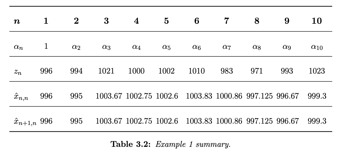
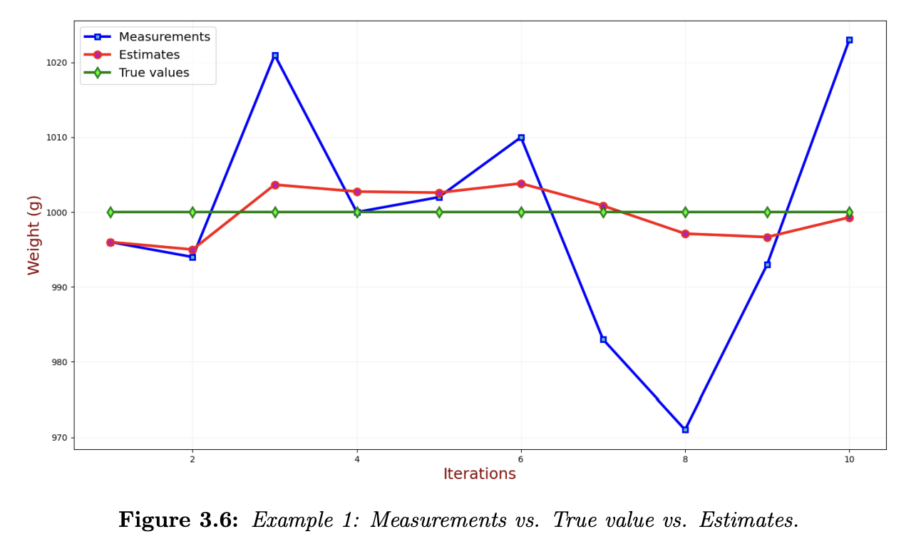
The following chart compares the true, measured, and estimated values. The estimation algorithm has a smoothing effect on the measurements and converges toward the true value.

In this example, we’ve developed a simple estimation algorithm for a static system. We have also derived the state update equation, one of the five Kalman Filter equations.