UDL Chapter 8 Problems

Problem 8.1

Will the multiclass cross-entropy loss in figure 8.2 ever reach zero? Explain your reasoning.

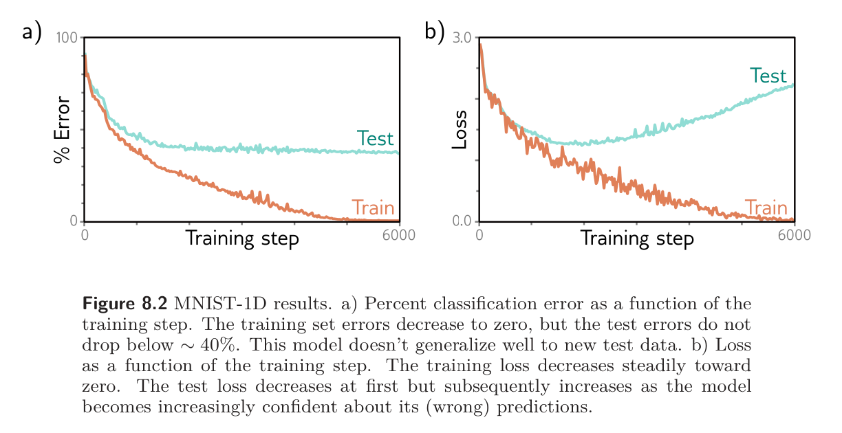
In multi-class classification, the likelihood that input $\mathbf{x}$ has label $y=k$ is:

$$Pr(y=k|\mathbf{x})={\text{softmax}}_k[f[\mathbf{x},\varphi ]]$$

and the loss function is the negative log-likelihood of the training data:

$$\begin{array}{rl}L[\varphi ]& =-\sum _{i=1}^I\log \left[{\text{softmax}}_{y_i}\right[f[{\mathbf{x}}_{\mathbf{i}},\varphi ]\left]\right]\end{array}$$

Thus, for the loss to be zero, we need ${\text{softmax}}_{y_i}[f[{\mathbf{x}}_{\mathbf{i}},\varphi ]]$ to be $1$. This is impossible as $\text{softmax}[z]=1$ only for $z\to \infty$. With any finite parameters, we will have $\text{softmax}[z]<1$. Thus, although we can get arbitrarily close to zero, we will never get exactly zero.

Problem 8.2

What values should we choose for the three weights and biases in the first layer of the model in figure 8.4a so that the hidden unit’s responses are as depicted in figures 8.4b–d?

• The weights should all be $1$.
• First bias: $0$
• Second bias: $-\frac{1}{3}$
• Third bias: $-\frac{2}{3}$

Problem 8.3

Given a training dataset consisting of $I$ input/output pairs $\{x_i,y_i\}$, show how the parameters $\{\beta ,{\omega }_1,{\omega }_2,{\omega }_3\}$ for the model in figure 8.4a using the least squares loss function can be found in closed form.

The first part of the network is deterministic since we’ve fixed the weights and the biases between the input and the first hidden layer. Thus, we can compute the activations at the hidden units for any input. Denoting these by $h_1,h_2,h_3$, we can write out the output layer now have a linear regression problem:

$$y_i=\beta +{\omega }_1{h}_{1i}+{\omega }_2{h}_{2i}+{\omega }_3{h}_{3i}$$

where $i$ indexes the training data. This can be solved in closed form with Ordinary Least Squares for example.

Problem 8.4

Consider the curve in figure 8.10b at the point where we train a model with a hidden layer of size 200, which would have 50,410 parameters. What do you predict will happen to the training and test performance if we increase the number of training examples from 10,000 to 50,410.

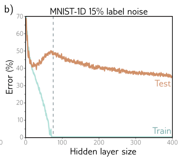
The training performance would be worse than before, as the number of model parameters compared to training examples is less than before, making the training set harder to memorize. However, testing performance may be better; with more data, variance decreases, resulting in less test error. One can also argue that noise, while irreducible, is diluted in this case because the model can rely on more clean samples.

Problem 8.5

Consider the case where the model capacity exceeds the number of training data points, and the model is flexible enough to reduce the training loss to zero. What are the implications of this for fitting a heteroscedastic model? Propose a method to resolve any problems that you identify.

Recall that heteroscedastic means that the uncertainty of the model varies as a function of input data.

In this case, we would typically predict the variance as a model output in the training process. However, if we are overparametrized, there are no residuals to train the variance on, so the variance would always be zero.

Some ways to deal with this would be to compute residuals on held-out predictions and train the variance on those instead of in-sample points. Or, we could constrain by putting some floor variance. The obvious best thing to do would be regularization to keep the model from perfectly fitting but the point here is to overfit I think.

Problem 8.6

Show that two random points drawn from a 1000-dimensional Gaussian distribution are orthogonal relative to the origin with high probability.

Let $X,Y\in {\mathbb{R}}^d$ be independent with $X,Y\sim \mathcal{N}(0,I_d)$, taking $d=1000$. The angle between them is

$$\cos \theta =\frac{X\cdot Y}{||X||||Y||}$$

Gaussian vectors are rotationally invariant. We can rotate coordinates so that the unit vectors in the direction of $Y$ is $e_1$. Then

$$\cos \theta =\frac{X}{||X||}\cdot e_1=U_1$$

where $U:=X/||X||$ is a uniform random point on the unit sphere $S^{d-1}$ and $U_1$ is its first coordinate. So, the problem reduces to understanding the first coordinate of a random unit vector.

By symmetry, $\mathbb{E}[U_1]=0$. Also, since ${\sum }_{i=1}^d{U}_i^2=1$ and all coordinates are identically distributed,

$$\mathbb{E}[U_1^2]=\frac{1}{d}$$

Thus

$$\mathbb{E}[\cos \theta ]=0,\text{Var}(\cos \theta )=\frac{1}{d}$$

Thus, a typical size of $|\cos \theta |$ is $\frac{1}{\sqrt{d}}$. For $d=1000$, that’s about $0.032$, so the two points are nearly orthogonal.

Problem 8.7

The volume of a hypersphere with radius $r$ in $D$ dimensions is:

$$\text{Vol}[r]=\frac{r^D{\pi }^{D/2}}{\Gamma [D/2+1]}$$

where $\Gamma [\bullet ]$ is the Gamma Function. Show using Stirling’s Formula that the volume of a hypersphere of diameter one (radius $r=0.5$) becomes zero as dimension increases.

Let $D$ be the dimension and $r=\frac{1}{2}$. Write $n:=\frac{D}{2}$. The volume is

$$\text{Vol}\left[\frac{1}{2}\right]=\frac{(1/2{)}^D{\pi }^{D/2}}{\Gamma (D/2+1)}=\frac{(\pi /4{)}^n}{\Gamma (n+1)}$$

Using Stirling’s formula gives us:

$$\Gamma (n+1)\approx x!\approx \sqrt{2\pi n}{\left(\frac{n}{e}\right)}^n$$

Hence:

$$\text{Vol}\left[\frac{1}{2}\right]=\frac{1}{\sqrt{2\pi n}}{\left(\frac{e\pi }{4n}\right)}^n$$

As $n\to \infty$ , we will have ${\left(\frac{e\pi }{4n}\right)}^n\to 0$. Therefore:

$$\text{Vol}\left[\frac{1}{2}\right]\to 0\text{as}D\to \infty$$

Problem 8.8

Consider a hypersphere of radius $r=1$. Find an expression for the proportion of the total volume that lies in the outermost 1% of the distance from the center (i.e., in the outermost shell of 0.01). Show that this becomes one as the dimension increases.

The volume is given by:

$$\text{Vol}[1]=\frac{{\pi }^{D/2}}{\Gamma [D/2+1]}$$

Volume of a hypersphere of radius $r=0.99$ is given by:

$$\text{Vol}[0.99]=\frac{0.99^D{\pi }^{D/2}}{\Gamma [D/2+1]}$$

The proportion $p$ in the last percentage is hence:

$$p=\frac{\text{Vol}[1]-\text{Vol}[0.99]}{\text{Vol}[1]}=1-0.99^D$$

We have $p\to 1$ as $D\to \infty$.

Problem 8.9

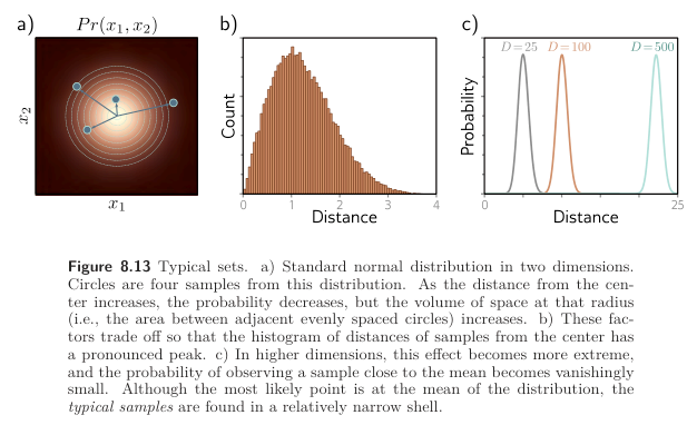
Figure 8.13c shows the distribution of distances of samples of a standard normal distribution as the dimension increases. Empirically verify this finding by sampling from the standard normal distributions in 25, 100, and 500 dimensions and plotting a histogram of the distances from the center. What closed-form probability distribution describes these distances?

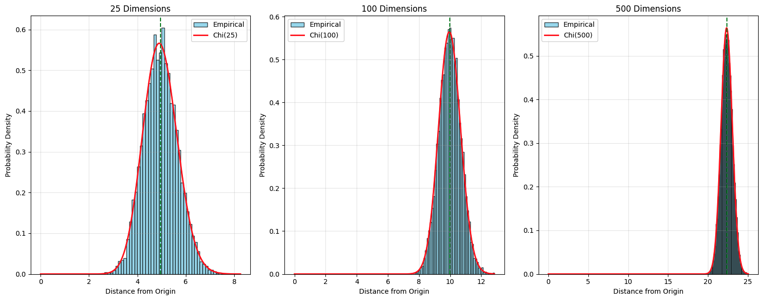
25 Dimensions:

• Mean distance: 4.9506
• Std distance: 0.7010
• Theoretical mean: 6.2666

100 Dimensions:

• Mean distance: 9.9846
• Std distance: 0.7034
• Theoretical mean: 12.5331

500 Dimensions:

• Mean distance: 22.3492
• Std distance: 0.7029
• Theoretical mean: 28.0250

The distances from the origin of samples from standard normal distributions follow a Chi distribution with degrees of freedom equal to the number of dimensions.

Key properties:

• Mean $d\approx \sqrt{n}$ for large $n$
• The distribution becomes more concentrated around $\sqrt{n}$ as $n$ increases
• This is the theoretical foundation for the curse of dimensionality.