Composing Shallow Networks

As an entrypoint to deep neural networks, we first consider composing two shallow neural networks so that the output of the first becomes the input of the second.

Consider two shallow networks with 3 hidden units each.

The first network takes an input $x$ and returns output $y$ and is defined by:

$$\begin{array}{r}{h}_1=a[{\theta }_{10}+{\theta }_{11}x]\\ h_2=a[{\theta }_{20}+{\theta }_{21}x]\\ h_3=a[{\theta }_{30}+{\theta }_{31}x]\end{array}$$

and

$$y={\varphi }_0+{\varphi }_1{h}_1+{\varphi }_2{h}_2+{\varphi }_3{h}_3$$

The second network takes $y$ as input and returns $y^{\prime }$ and is defined by:

$$\begin{array}{r}{h}_1^{\prime }=a[{\theta }_{10}^{\prime }+{\theta }_{11}^{\prime }y]\\ h_2^{\prime }=a[{\theta }_{20}^{\prime }+{\theta }_{21}^{\prime }y]\\ h_3^{\prime }=a[{\theta }_{30}^{\prime }+{\theta }_{31}^{\prime }y]\end{array}$$

and

$$y^{\prime }={\varphi }_0^{\prime }+{\varphi }_1^{\prime }{h}_1^{\prime }+{\varphi }_2^{\prime }{h}_2^{\prime }+{\varphi }_3^{\prime }{h}_3^{\prime }$$

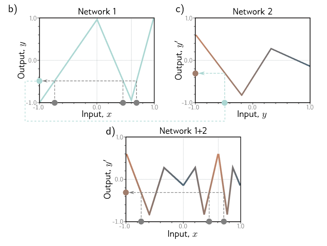
• The first network maps inputs $x\in [-1,1]$ to outputs $y\in [-1,1]$ using a function comprising three linear regions that are chosen so that they alternate the sign of their slope (4th linear region is outside range of graph). Multiple inputs $x$ (gray circles) now map to the same output $y$ (cyan circle).
• The second network defines a function comprising three linear regions that takes $y$ and returns $y^{\prime }$ (i.e. the cyan circle is mapped to the brown circle).
• The combined effect of these 2 functions when composed is that three different inputs $x$ are mapped to any given value of $y$ by the first network and are processed the same way by the second network.
• The result is that the function defined by the second network in panel (c) is duplicated three times, variously flipped and rescaled according to the slope of the regions of panel (b).

With ReLU activations, this model also describes a family of piecewise linear functions. However, the number of linear regions is potentially greater than for a shallow network with 6 hidden units. To see this, consider choosing the first network to produce three alternating regions of positive and negative slope (panel b above). This means that three different ranges of $x$ are mapped to the same output range $y\in [-1,1]$, and the subsequent mapping from this range of $y$ to $y^{\prime }$ is applied three times. The overall effect is that the function defined by the second network is duplicated three times to create nine linear regions.

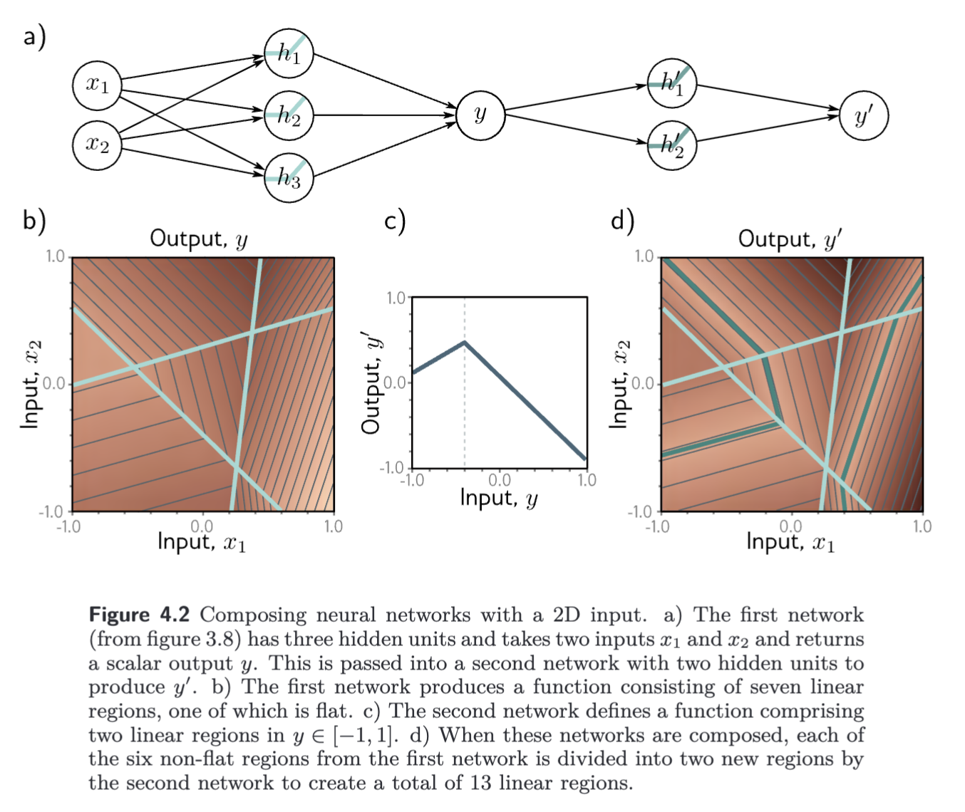
The same principle applies in higher dimensions as well.

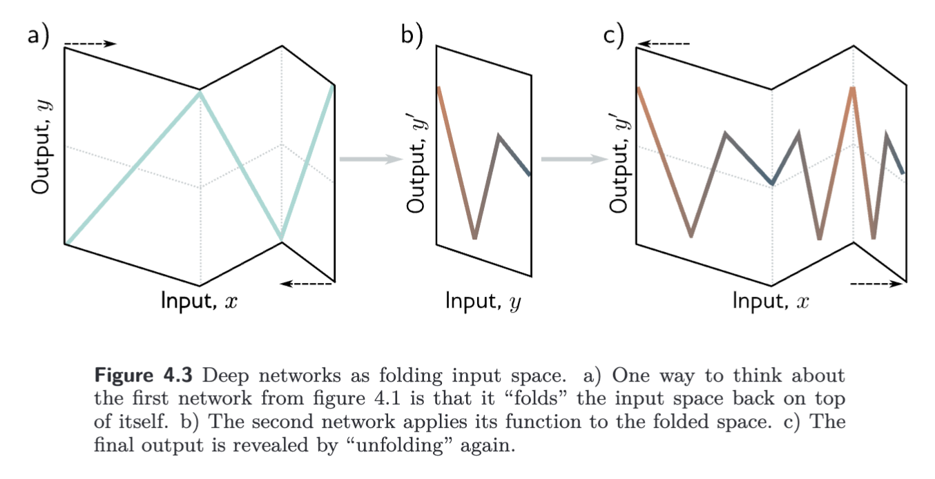
A different way to think about composing networks is that the first network “folds” input space $x$ onto itself so that multiple inputs generate the same output. Then the second network applies a function, which is replicated at all points that were folded on top of one another.

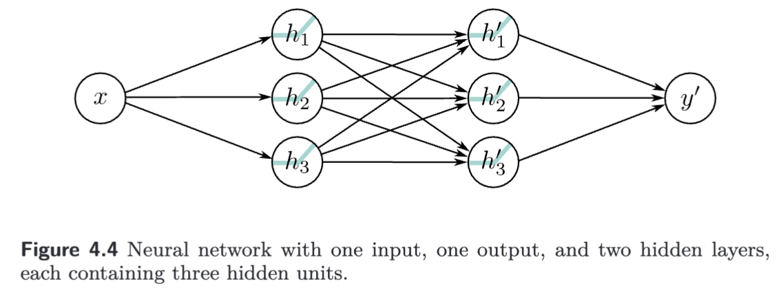
From composing networks to deep networks

We can show that our composition of networks is a special case of a Deep Neural Network with two hidden layers. The first layer is defined by

$$\begin{array}{rl}{h}_1& =a[{\theta }_{10}+{\theta }_{11}x]\\ h_2& =a[{\theta }_{20}+{\theta }_{21}x]\\ h_3& =a[{\theta }_{30}+{\theta }_{31}x]\end{array}$$

The output of the first network ($y={\varphi }_0+{\varphi }_1{h}_1+{\varphi }_2{h}_2+{\varphi }_3{h}_3$) is a linear combination of the activations of the hidden units. The first operations of the second network (${\theta }_{10}^{\prime }+{\theta }_{11}^{\prime }y,{\theta }_{20}^{\prime }+{\theta }_{21}^{\prime }y,{\theta }_{30}^{\prime }+{\theta }_{31}^{\prime }y$) are linear in the output of the first network. Applying one linear function to another yields another linear function.

Substituting the expression for $y$ in the calculation of hidden units in the second network gives:

$$\begin{array}{r}{h}_1^{\prime }=a[{\theta }_{10}^{\prime }+{\theta }_{11}^{\prime }y]=a[{\theta }_{10}^{\prime }+{\theta }_{11}^{\prime }{\varphi }_0+{\theta }_{11}^{\prime }{\varphi }_1{h}_1+{\theta }_{11}^{\prime }{\varphi }_2{h}_2+{\theta }_{11}^{\prime }{\varphi }_3{h}_3]\\ h_2^{\prime }=a[{\theta }_{20}^{\prime }+{\theta }_{21}^{\prime }y]=a[{\theta }_{20}^{\prime }+{\theta }_{21}^{\prime }{\varphi }_0+{\theta }_{21}^{\prime }{\varphi }_1{h}_1+{\theta }_{21}^{\prime }{\varphi }_2{h}_2+{\theta }_{21}^{\prime }{\varphi }_3{h}_3]\\ h_3^{\prime }=a[{\theta }_{30}^{\prime }+{\theta }_{31}^{\prime }y]=a[{\theta }_{30}^{\prime }+{\theta }_{31}^{\prime }{\varphi }_0+{\theta }_{31}^{\prime }{\varphi }_1{h}_1+{\theta }_{31}^{\prime }{\varphi }_2{h}_2+{\theta }_{31}^{\prime }{\varphi }_3{h}_3]\end{array}$$

which can be re-written as:

$$\begin{array}{r}{h}_1^{\prime }=a[{\psi }_{10}+{\psi }_{11}{h}_1+{\psi }_{12}{h}_2+{\psi }_{13}{h}_3]\\ h_2^{\prime }=a[{\psi }_{20}+{\psi }_{21}{h}_1+{\psi }_{22}{h}_2+{\psi }_{23}{h}_3]\\ h_3^{\prime }=a[{\psi }_{30}+{\psi }_{31}{h}_1+{\psi }_{32}{h}_2+{\psi }_{33}{h}_3]\end{array}$$

where ${\psi }_{10}={\theta }_{10}^{\prime }+{\theta }_{11}^{\prime }{\varphi }_0,{\psi }_{11}={\theta }_{11}^{\prime }{\varphi }_1,{\psi }_{12}={\theta }_{11}^{\prime }{\varphi }_2$ and so on. Finally we can define the output by:

$$y^{\prime }={\varphi }_0^{\prime }+{\varphi }_1^{\prime }{h}_1^{\prime }+{\varphi }_2^{\prime }{h}_2^{\prime }+{\varphi }_3^{\prime }{h}_3^{\prime }$$

The result is a network with two hidden layers.

It follows that a network with two layers can represent the family of functions created by passing the output of one single-layer network into another. It represents a broader family, because the nine slope parameters, ${\psi }_{11},{\psi }_{21},\dots ,{\psi }_{33}$ can take arbitrary values, whereas the original parameters are constrained to be the outer product $[{\theta }_{11}^{\prime },{\theta }_{21}^{\prime },{\theta }_{31}^{\prime }{]}^T[{\varphi }_1,{\varphi }_2,{\varphi }_3]$.

Considering the above equations leads to another way of thinking about how the network constructs an increasingly complex function:

1. The three hidden units $h_1,h_2$ and $h_3$ in the first layer are computed as usual by forming linear functions of the input and passing these through ReLU activation functions.
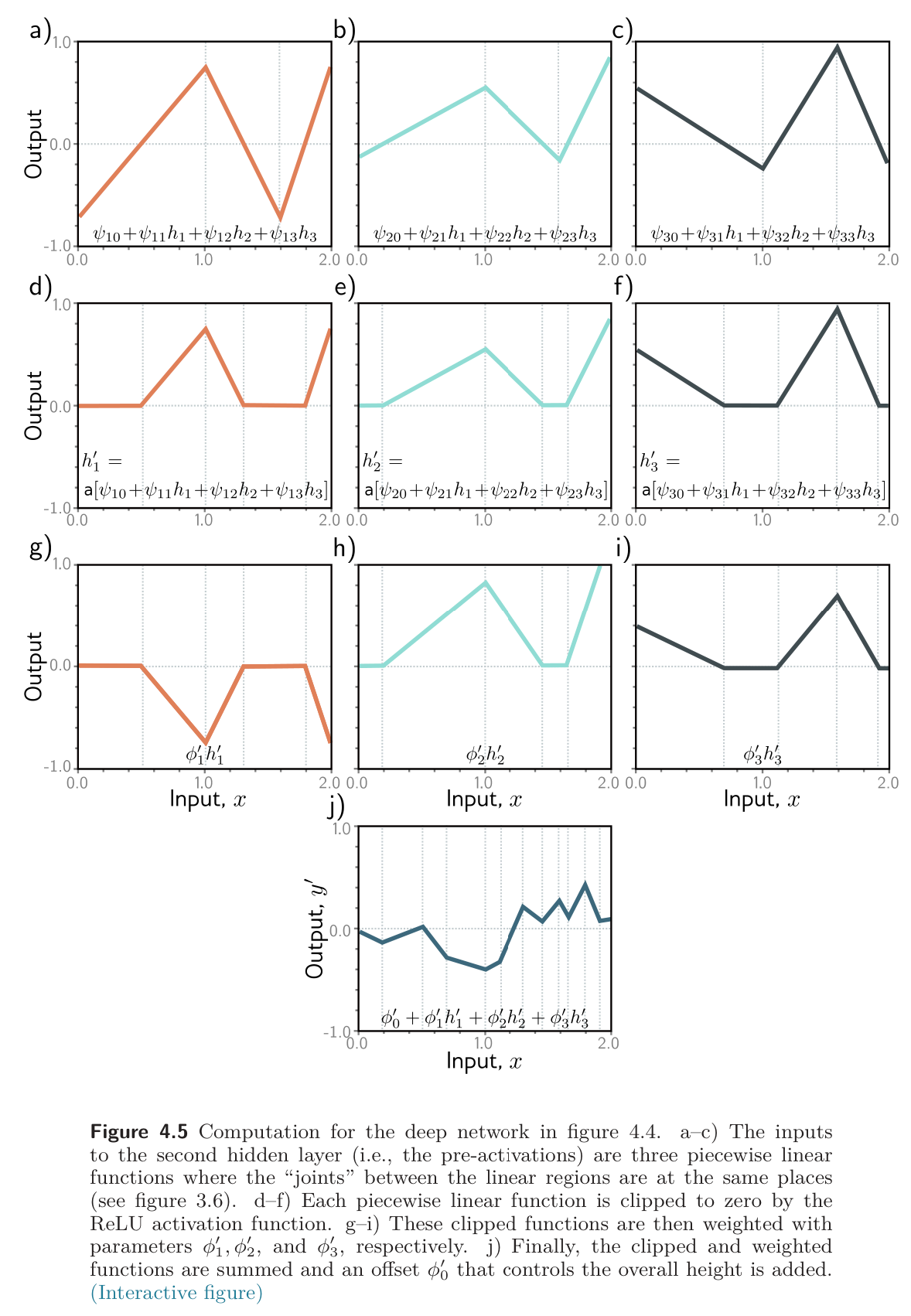
2. The pre-activations at second layer are computed by taking three new linear functions of these hidden units. At this point, we effectively have a shallow network with three outputs; we have computed three piecewise linear functions with the “joints” between linear regions in the same places.
3. At the second hidden layer, another ReLU function is applied to each function, which clips them and adds new “joints” to each.
4. The final output is a linear combination of these hidden units.

We can think of each layer as “folding” the input space or as creating the new functions, which are clipped (creating new regions) and then recombined. The former view emphasizes the dependencies in the output, but not how clipping creates new joints, and the latter has the opposite emphasis. Both only provide partial insight into how deep neural networks operate.

It’s important to not lose sight of the fact that this is still merely an equation relating input $x$ to output $y^{\prime }$. We can combine all the equations to get one expression:

$$\begin{array}{rl}{y}^{\prime }={\varphi }_0^{\prime }& +{\varphi }_1^{\prime }a[{\psi }_{10}+{\psi }_{11}a[{\theta }_{10}+{\theta }_{11}x]+{\psi }_{12}a[{\theta }_{20}+{\theta }_{21}x]+{\psi }_{13}a[{\theta }_{30}+{\theta }_{31}x]]\\ & +{\varphi }_2^{\prime }a[{\psi }_{20}+{\psi }_{21}a[{\theta }_{10}+{\theta }_{11}x]+{\psi }_{22}a[{\theta }_{20}+{\theta }_{21}x]+{\psi }_{23}a[{\theta }_{30}+{\theta }_{31}x]]\\ & +{\varphi }_3^{\prime }a[{\psi }_{30}+{\psi }_{31}a[{\theta }_{10}+{\theta }_{11}x]+{\psi }_{32}a[{\theta }_{20}+{\theta }_{21}x]+{\psi }_{33}a[{\theta }_{30}+{\theta }_{31}x]]\end{array}$$

Matrix Notation

We can describe our composition above in matrix notation as:

$$\left[\begin{array}{c}{h}_1\\ h_2\\ h_3\end{array}\right]=a\left[\begin{array}{c}\left[\begin{array}{c}{\theta }_{10}\\ {\theta }_{20}\\ {\theta }_{30}\end{array}\right]+\left[\begin{array}{c}{\theta }_{11}\\ {\theta }_{21}\\ {\theta }_{31}\end{array}\right]x\end{array}\right]$$

and

$$\left[\begin{array}{c}{h}_1^{\prime }\\ h_2^{\prime }\\ h_3^{\prime }\end{array}\right]=a\left[\begin{array}{c}\left[\begin{array}{c}{\psi }_{10}\\ {\psi }_{20}\\ {\psi }_{30}\end{array}\right]+\left[\begin{array}{ccc}{\psi }_{11}& {\psi }_{12}& {\psi }_{13}\\ {\psi }_{21}& {\psi }_{22}& {\psi }_{23}\\ {\psi }_{31}& {\psi }_{32}& {\psi }_{33}\end{array}\right]\left[\begin{array}{c}{h}_1\\ h_2\\ h_3\end{array}\right]\end{array}\right]$$

and

$$y^{\prime }={\varphi }_0^{\prime }+\left[\begin{array}{ccc}{\varphi }_1^{\prime }& {\varphi }_2^{\prime }& {\varphi }_3^{\prime }\end{array}\right]\left[\begin{array}{c}{h}_1^{\prime }\\ h_2^{\prime }\\ h_3^{\prime }\end{array}\right]$$

or even more compactly as

$$\begin{array}{rl}\mathbf{h}& =a[{\theta }_0+\theta x]\\ {\mathbf{h}}^{\prime }& =a[{\psi }_0+\Psi \mathbf{h}]\\ y^{\prime }& ={\varphi }_0^{\prime }+{\varphi }^{\prime }{\mathbf{h}}^{\prime }\end{array}$$

where, in each case, the function $a[\cdot ]$ applies the activation function separately to every element of its vector input.