Shallow Neural Network

Shallow neural networks are functions $\mathbf{y}=\mathbf{f}[\mathbf{x},\varphi ]$ that map multi-dimensional inputs $\mathbf{x}\in {\mathbb{R}}^{D_i}$ to a multi-dimensional output $\mathbf{y}\in {\mathbb{R}}^{D_o}$ using $\mathbf{h}\in {\mathbb{R}}^D$ hidden units. Each hidden unit is computed as:

$$h_d=a\left[{\theta }_{d_0}+\sum _{i=1}^{D_i}{\theta }_{d_i}{x}_i\right]$$

which are combined linearly to create an output.

Intuition

We can illustrate the main ideas using an example network $f[x,\varphi ]$ that maps a scalar input $x$ to a scalar output $y$, using ten parameters $\varphi =\{{\varphi }_0,{\varphi }_1,{\varphi }_2,{\varphi }_3,{\theta }_{10},{\theta }_{11},{\theta }_{20},{\theta }_{21},{\theta }_{30},{\theta }_{31}\}$. This is defined such that:

$$\begin{array}{rl}y& =f[x,\varphi ]\\ & ={\varphi }_0+{\varphi }_{1}a[{\theta }_{10}+{\theta }_{11}x]+{\varphi }_{2}a[{\theta }_{20}+{\theta }_{21}x]+{\varphi }_{3}a[{\theta }_{30}+{\theta }_{31}x]\end{array}$$

This calculation can be broken down into three parts:

1. We compute three linear functions of the input data, ${\theta }_{10}+{\theta }_{11}x$, ${\theta }_{20}+{\theta }_{21}x$ and ${\theta }_{30}+{\theta }_{31}x$
2. We pass the three results through an activation function $a[\cdot ]$
3. We weight the three resulting activations with ${\varphi }_1$, ${\varphi }_2$ and ${\varphi }_3$, sum them, and then add an offset ${\varphi }_0$.

Equation $(1)$ characterizes a family of functions where the particular member of the family is characterized by the parameters $\varphi$. Given these parameters, we can perform inference to predict $y$ by evaluating the equation on a given $x$. Given a data set $\{x_i,y_i{\}}_{i=1}^I$, we can define a loss function $L[\varphi ]$ and use it to measure how effectively the model describes the data set for this given set of parameters $\varphi$. To train the model, we search for the values $\hat{\varphi }$ that minimize loss.

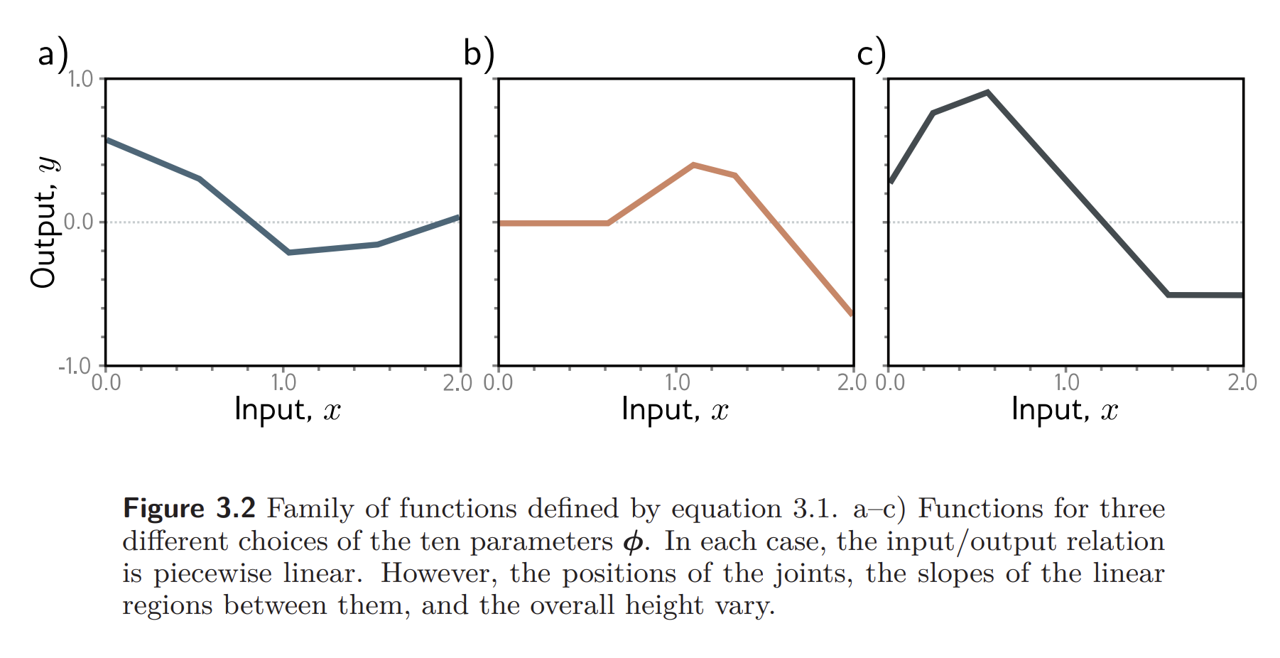
To gain more intuition, we can think about what equation $(1)$ actually represents. It is a family of piecewise functions with up to four linear regions. This can be easily seen by splitting up the quantities, which we call hidden units:

$$\begin{array}{r}{h}_1=a[{\theta }_{10}+{\theta }_{11}x]\\ h_2=a[{\theta }_{20}+{\theta }_{21}x]\\ h_3=a[{\theta }_{30}+{\theta }_{31}x]\end{array}$$

The output of then be found by combining these hidden units with a linear function:

$$y={\varphi }_0+{\varphi }_1{h}_1+{\varphi }_2{h}_2+{\varphi }_3{h}_3$$

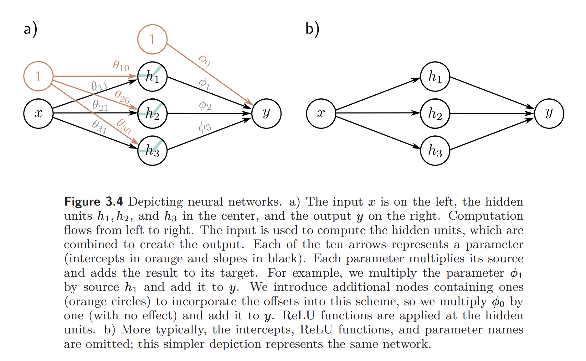
The flow of computation is shown here:

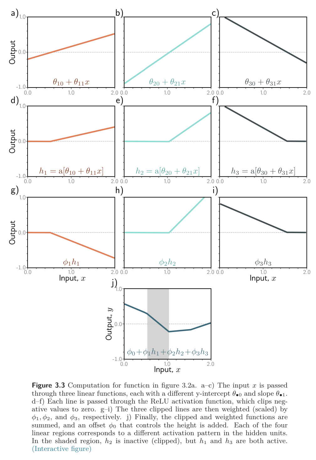
• Each hidden unit contains a linear function ${\theta }_{\bullet 0}+{\theta }_{\bullet 1}x$.
• This line is clipped by the ReLU $a[\bullet ]$ below zero.
• The positions where the three liens cross zero become the “joints” in the output.
• The three clipped lines are then weighted by ${\varphi }_1,{\varphi }_2,{\varphi }_3$.
• Finally, the offset ${\varphi }_0$ is added.

Each linear region corresponds to a different activation pattern in the hidden units. When a unit is clipped, its referred to as inactive; when it’s not clipped, we say it’s active.

• For example, the shaded region above has $h_1$ and $h_3$ active, while $h_2$ is inactive.

The slope of each linear region is determined by the original slopes ${\theta }_{\bullet 1}$ and the weights ${\varphi }_{\bullet }$ that were subsequently applied.

• For example, the slope in the shaded region is ${\varphi }_1{\theta }_{11}+{\varphi }_3{\theta }_{31}$, where the first term is the slope in panel (g) and the second is the slope in panel (i).

Each hidden unit contributes one “joint” to the function, so with three hidden units, there can be four linear regions. However, only three of the slopes of these regions are independent; the fourth is either zero (if all the hidden units are inactive in this region) or is a sum of slopes from the other regions.

Network Visualization

The network we’ve been discussing has one input, one output, and three hidden units. This can be depicted as such: