1D Normalizing Flows Intuition

Normalizing Flows are probabilistic generative models; they fit a probability distribution to training data.

Consider modeling a 1D distribution $Pr(x)$. Normalizing flows start with a simple tractable base distribution $Pr(z)$ over a latent variable $z$ and apply a function $x=f[z,\varphi ]$, where the parameters $\varphi$ are chosen so that $Pr(x)$ has the desired distribution. We can then easily generate a new example $x^{\ast }$; we draw $z^{\ast }$ from the base density and pass this through the function so that $x^{\ast }=f[z^{\ast },\varphi ]$.

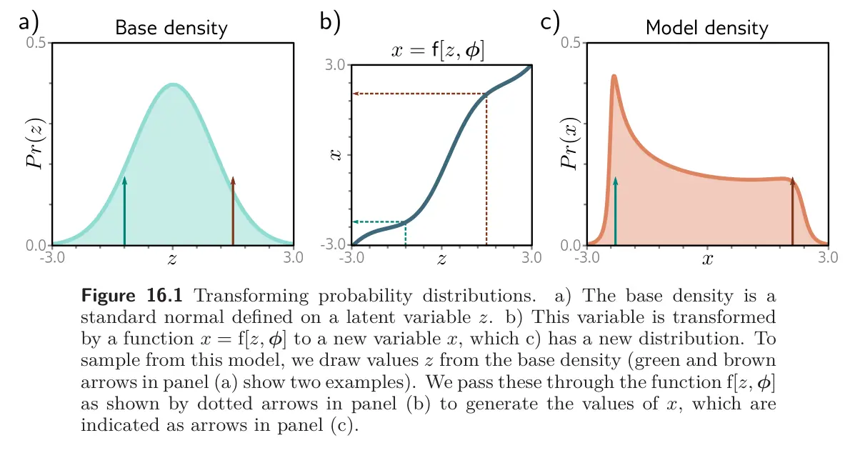
Measuring probability

Measuring the probability of a data point $x$ is more challenging. Consider applying a function $f[z,\varphi ]$ to a random variable with known density $Pr(z)$:

• The probability density will decrease in areas that are stretched by the function and increase in areas that are compressed so that the area under the under the new distribution remains one.
• The degree to which a function $f[z,\varphi ]$ stretches or compresses its input depends on the magnitude of its gradient.
• If a small change to the input causes a large change in the output, it stretches the function. If a small change to the input causes a smaller change in the output, it compresses the function.

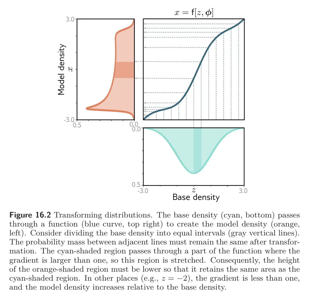
• Intuition: if a small region of the base density corresponds to a large region of the model density, the height of the model density’s large region must be smaller such that probability mass stays constant.

More precisely, the probability of data $x$ under the transformed distribution is:

$$Pr(x|\varphi )={\left|\frac{\partial f[z,\varphi ]}{\partial z}\right|}^{-1}\cdot Pr(z)$$

where $z=f^{-1}[x,\varphi ]$ is the latent variable that created $x$. The term $Pr(z)$ is the original probability of this latent variable under the base density. This is moderated according to the magnitude of the derivative of the function. If it is greater than one, the probability decreases; if it is smaller, the probability increases.

Forward and inverse mappings

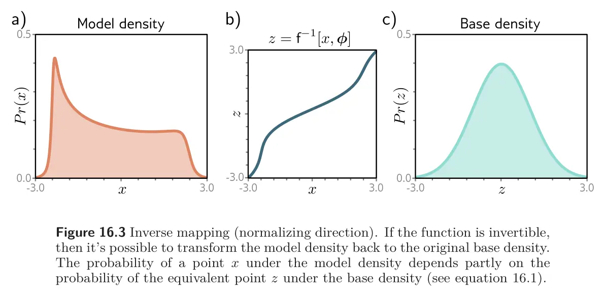
To draw samples form the distribution, we need the forward mapping $x=f[z,\varphi ]$, but to measure the likelihood, we need to compute the inverse $z=f^{-1}[x,\varphi ]$. Hence, we need to choose $f[z,\varphi ]$ so that it is invertible.

• The forward mapping is sometimes called the generative direction.
• The base density is usually chosen to be a standard normal distribution. Hence, the inverse mapping is called the normalizing direction since this takes the complex distribution over $x$ and turns it into a normal distribution over $z$.

Learning

To learn the distribution, we find parameters $\varphi$ that maximize the likelihood of the training data $\{x_i{\}}_{i=1}^I$ or equivalently minimize the negative log-likelihood:

$$\begin{array}{rl}\hat{\varphi }& =\underset{\varphi }{\mathrm{argmax}}\left[\prod _{i=1}^{I}Pr(x_i|\varphi )\right]\\ & =\underset{\varphi }{\mathrm{argmin}}\left[\sum _{i=1}^I-\log [Pr(x_i|\varphi )]\right]\\ & =\underset{\varphi }{\mathrm{argmin}}\left[\sum _{i=1}^I\log \left[\left|\frac{\partial f[z_i,\varphi ]}{\partial z}\right|\right]-\log [Pr(z_i)]\right]\end{array}$$

where we have assumed that the data are independent and identically distributed in the first line and used the likelihood equation from above in the third line.

Essentially, during training, we observe $x_i$, and then calculate $z=f^{-1}[x_i,\varphi ]$ (hence the requirement for invertible layers) so that we can calculate the $\frac{\partial f[z_i,\varphi ]}{\partial z}$ and $Pr(z_i)$ terms.