Residual Flows

iRevNet

Residual flows take inspiration from residual networks. They divide the input into two parts $h=h[h_1^T,h_2^T{]}^T$ (similar to coupling flows) and define the outputs as:

$$\begin{array}{rl}{h}_1^{\prime }& =h_1+f_1[h_2,{\varphi }_1]\\ h_2^{\prime }& =h_2+f_2[h_1^{\prime },{\varphi }_2]\end{array}$$

where $f_1$ and $f_2$ are two functions that do not necessarily have to be invertible. The inverse can be computed by reversing the order of computation:

$$\begin{array}{rl}{h}_2& =h_2^{\prime }-f_2[h_1^{\prime },{\varphi }_2]\\ h_1& =h_1^{\prime }-f_1[h_2,{\varphi }_1]\end{array}$$

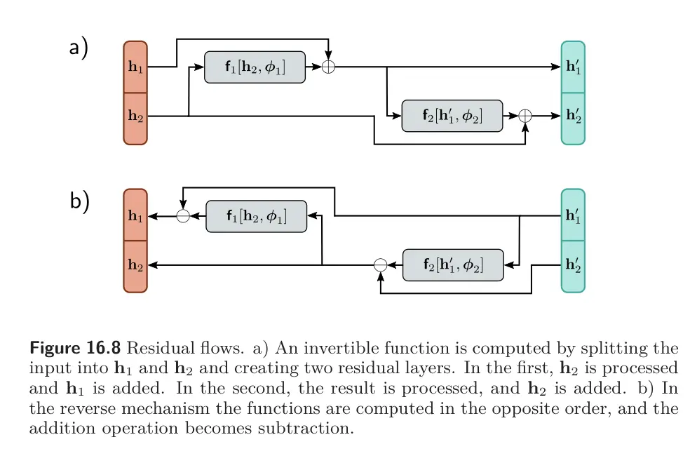
As for coupling flows, the division into blocks restricts the family of transformations that can be represented. Thus, the inputs are permuted between layers so that the variables can mix in arbitrary ways.

This formulation can be inverted easily, but for general functions $f_1[\bullet ,{\varphi }_1]$ and $f_2[\bullet ,{\varphi }_2]$, there is no efficient way to compute the Jacobian.

This formulation is sometimes used to save memory when training residual networks; because the network is invertible, storing the activations at each layer in the forward pass is unnecessary.

iResNet

Another approach to exploit residual networks is to utilize the Banach fixed point theorem or contraction mapping theorem, which states that every contraction mapping has a fixed point. A contraction mapping $f[\bullet ]$ has the property that:

$$\text{dist}[f[z^{\prime }],f[z]]<\beta \bullet \text{dist}[z^{\prime },z]\forall z,z^{\prime }$$

where $\text{dist}[\bullet ,\bullet ]$ is a distance function and $0<\beta <1$. When a function with this property is iterated (i.e., the output is repeatedly passed back in as an input), the result converges to a fixed point where $f[z]=z$.

• To understand this, consider applying the function to both the fixed point and the current position; the fixed point remains static, but the distance between the two must become smaller, so the current position must get closer to the fixed point.

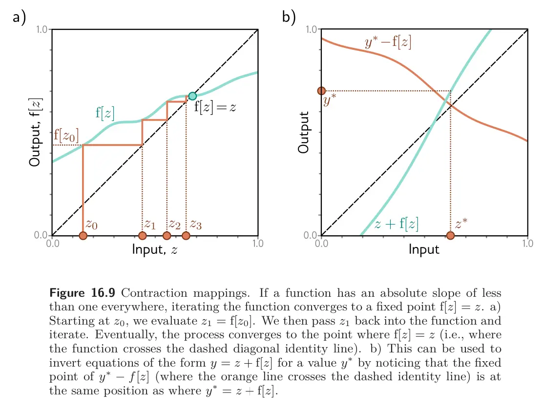
The theorem can be exploited to invert an equation of the form:

$$y=z+f[z]$$

if $f[z]$ is a contraction mapping. In other words, it can be used to find the $z^{\ast }$ that maps to a given value, $y^{\ast }$. This can be done by starting with any point $z_0$ and iterating $z_{k+1}=y^{\ast }-f[z_k]$. This has a fixed point at $z+f[z]=y^{\ast }$.

The same principle can be used to invert residual network layers of the form $h^{\prime }=h+f[h,\varphi ]$ if we ensure that $f[h,\varphi ]$ is a contraction mapping. In practice, this means that the Lipschitz constant must be less than one. Assuming that the slope of the activation functions is not greater than one, this is equivalent to ensuring that the largest eigenvalue of each weight matrix $\Omega$ must be less than one. A crude way to do this is to ensure that the absolute magnitudes of the weights $\Omega$ are small by clipping them.

The Jacobian determinant cannot be computed easily, but its logarithm can be approximated using a series of tricks:

$$\begin{array}{rl}\log \left[\left|I+\frac{\partial f[h,\varphi ]}{\partial h}\right|\right]& =\text{trace}\left[\log \left[I+\frac{\partial f[h,\varphi ]}{\partial h}\right]\right]\\ & =\sum _{k=1}^{\infty }\frac{(-1{)}^{k-1}}{k}\text{trace}{\left[\frac{\partial f[h,\varphi ]}{\partial h}\right]}^k\end{array}$$

where we have used the identity $\log [\left|A\right|]=\text{trace}[\log [A]]$ in the first line, and expanded this into a power series in the second line.

Even when we truncate this series, it’s still computationally expensive to compute the trace of the constituent terms. Hence, we approximate this using Hutchinson’s trace estimator. Consider a normal random variable $ϵ$ with mean $0$ and variance $I$. The trace of a matrix $A$ can be estimated as:

$$\begin{array}{rl}\text{trace}[A]& =\text{trace}[A\mathbb{E}[ϵ{ϵ}^T]]\\ & =\text{trace}[\mathbb{E}[Aϵ{ϵ}^T]]\\ & =\mathbb{E}[\text{trace}[Aϵ{ϵ}^T]]\\ & =\mathbb{E}[\text{trace}[{ϵ}^{T}Aϵ]]\\ & =\mathbb{E}[{ϵ}^{T}Aϵ]\end{array}$$

where:

• The first line is true because $\mathbb{E}[ϵ{ϵ}^T]=I$.
• The second line derives from the properties of the expectation operator.
• The third line comes form the linearity of the trace operator.
• The fourth line is due to the invariance of the trace to cyclic permutation
• The final line is true because the argument in the fourth line is now a scalar.

We estimate the trace by drawing samples ${ϵ}_i$ from $Pr(ϵ)$:

$$\begin{array}{rl}\text{trace}[A]& =\mathbb{E}[{ϵ}^{T}Aϵ]\\ & =\frac{1}{I}\sum _{i=1}^I{ϵ}_i^{T}A{ϵ}_i\end{array}$$

In this way, we can approximate the trace of the powers of the Taylor expansion and evaluate the log probability.