Graph Neural Networks

Graph neural networks are architectures that process graphs (i.e., sets of nodes connected by edges).

Graphs are hard to process for three reasons:

1. Their topology is variable; it’s hard to design networks that are both sufficiently expressive and can cope with this variation.
2. Graphs may be enormous; a graph representing connections in a social network might have a billion nodes.
3. There may only be a single monolithic graph available, so the usual protocol of training with many data examples and testing with new data is not always appropriate.

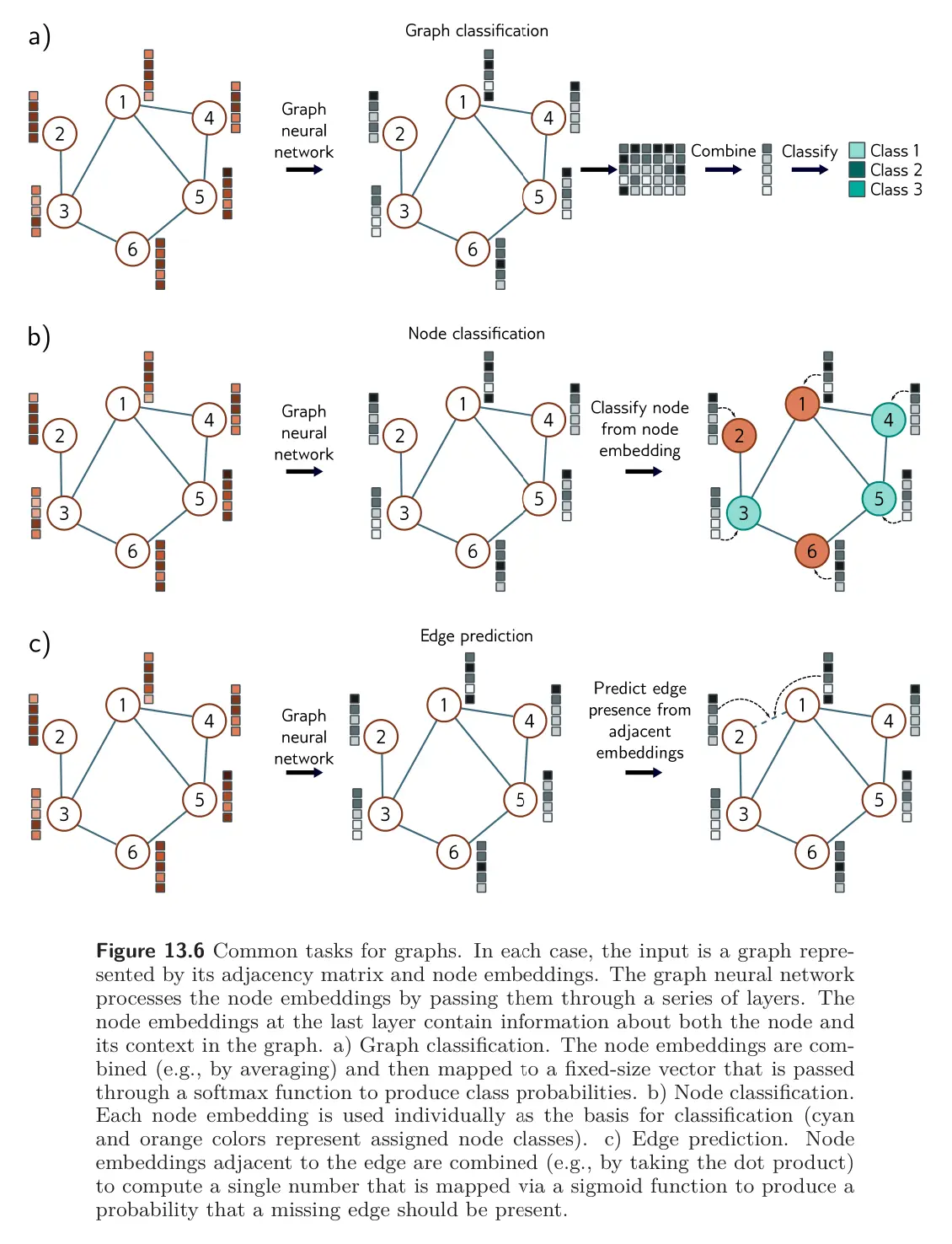
Given a graph representation, a graph neural network takes the node embeddings $\mathbf{X}$ and the adjacency matrix $\mathbf{A}$ as inputs and passes them through a series of $K$ layers. The node embeddings are updated at each layer to create intermediate “hidden” representations ${\mathbf{H}}_k$ before finally computing output embeddings ${\mathbf{H}}_K$.

At the start of the network, each column of the input node embeddings $\mathbf{X}$ just contains information about the node itself. At the end, each column of the model output ${\mathbf{H}}_K$ includes information about the node and its context within the graph. This is similar to word embeddings passing through a transformer, where the embeddings represent words at the start but represent meanings in the context of the sentence at the end.

A common architecture is the Graph Convolutional Network.

Tasks and loss function

Supervised graph problems usually fall into one of three categories.

Graph-level tasks

The network assigns a label or estimates some values from the to the entire graph, exploiting both the structure and the node embeddings.

• Examples: Predict the temperature at which a molecule becomes liquid (regression task), whether a molecule is poisonous to humans (classification task)

For graph-level tasks, the output node embeddings are combined (e.g., by averaging), and mapped via a linear transformation to a fixed-size vector. For regression, the residual between the result and the ground truth value is computed using a least squares loss.

For binary classification, the output is passed through a sigmoid, and the mismatch is calculated via binary cross-entropy loss. Here, the probability that the graph belongs to class one might be:

$$\text{Pr}(y=1|\mathbf{X},\mathbf{A})=\text{sig}[{\beta }_K+{\omega }_K{\mathbf{H}}_{k}1/N]$$

where the scalar ${\beta }_K$ and the $1\times D$ vector ${\omega }_K$ are learned parameters. Post-multiplying the output embeddings ${\mathbf{H}}_K$ by the column vector $1$ sums together all the embeddings, and then dividing by $N$ gives the average. This is similar to mean pooling.

Node-level tasks

The network assigns a label (classification) or some values (regression) to each node of the graph.

• For example, given a graph constructed from a 3D point cloud of an airplane, the goal might be to classify the nodes according to whether they belong to the wings or the fuselage.

Loss functions are defined int he same way for graph-level tasks, except that now this is done independently at each node $n$:

$$\text{Pr}(y^n=1|\mathbf{X},\mathbf{A})=\text{sig}[{\beta }_K+{\omega }_K{\mathbf{h}}_k^n]$$

Edge prediction tasks

The network predicts whether or not there should be an edge between nodes $n$ or $m$.

• For example, in the social network setting, the network might predict whether two people know and like each other and suggest that they connect if that is the case.

This is a binary classification task where the two node embeddings must be mapped to a single number representing the probability that the edge is present. One way is to take the dot product of the node embeddings and pass the result through a sigmoid function to create the probability:

$$\text{Pr}(y^{(mn)}=1|\mathbf{X},\mathbf{A})=\text{sig}[{\mathbf{h}}^{(m)T}{\mathbf{h}}^{(n)}]$$