Consider a binary node classification task in a transductive setting.
We start with a commercial-sized graph with millions of nodes. Some nodes have ground truth binary labels, and the goal is to label the remaining unlabeled nodes. The body of the network will be the same as in the graph classification example but with a different final layer that produces an output vector of size :
where the function applies the sigmoid function independently to every element of the row input. We use binary cross-entropy loss, but now only at nodes where we know the ground truth label .
- Note that this is just a vectorized version of the basic node classification loss
Training this network has two problems:
- It’s logistically difficult to train a graph neural network of this size. We must store the node embeddings at every network layer in the forward pass. This will involve both storing and processing a structure several times the size of the entire graph (which is quite big).
- We only have a single graph, so it’s not obvious how to perform stochastic gradient descent. How can we form a batch if there is only a single object?
Batching methods
K-hop neighborhood
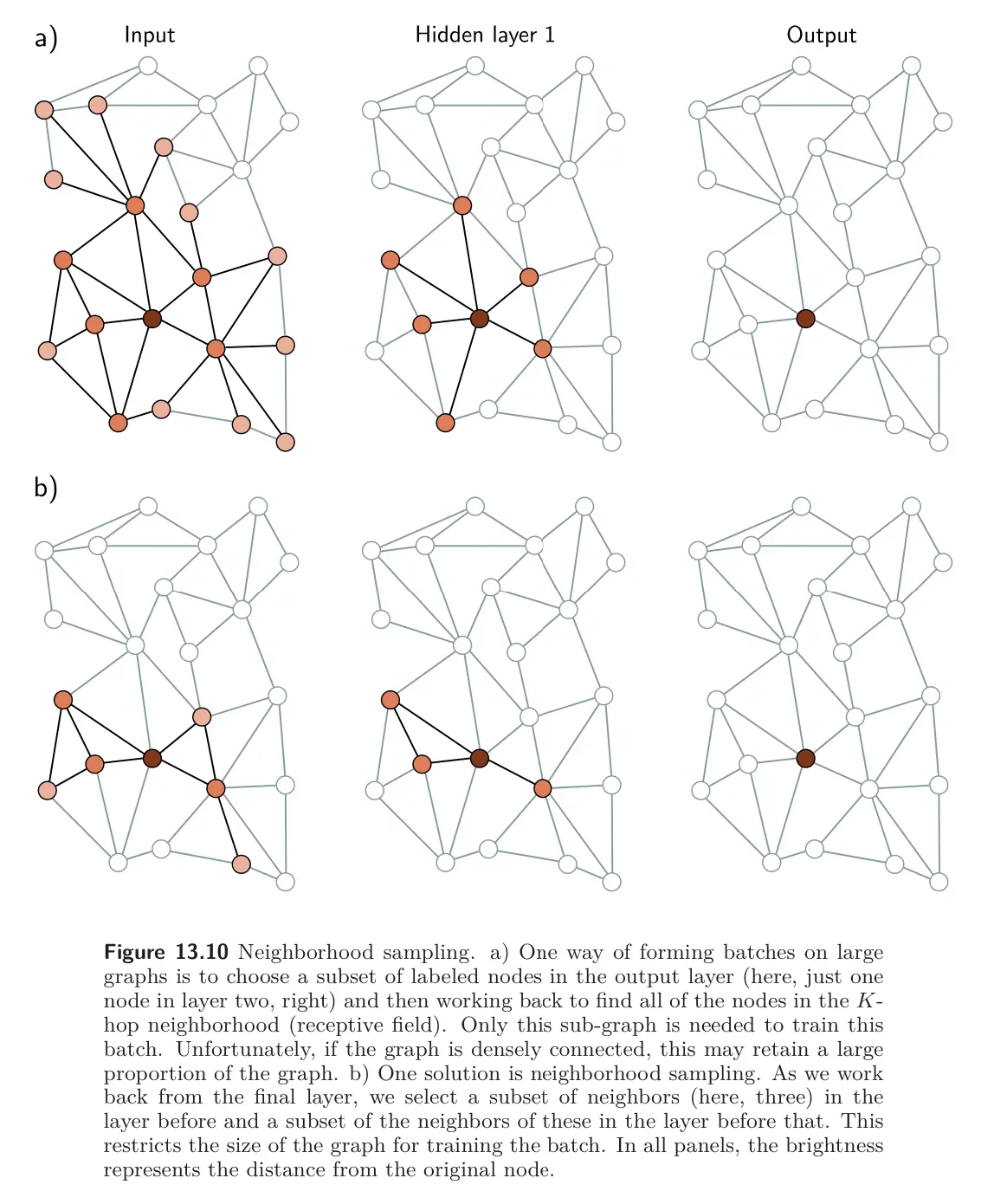
One way to form a batch is to choose a random subset of labeled nodes at each training step. In a GCN architecture, each node depends on its neighbors in the previous layer. These, in turn, depend on their neighbors in the layer before, so each node has a receptive field. The receptive is called the k-hop neighborhood. We can hence perform a gradient descent using the graph that forms the union of the k-hop neighborhoods of the batch nodes; the remaining inputs do not contribute.
Unfortunately if there are many layers and the graph is densely connected, every input node may be in the receptive field of every output, and this may not reduce the graph size at all. This is called the graph expansion problem. Two approaches that tackle this problem are neighborhood sampling and graph partitioning.
Neighborhood sampling
The full graph that feeds into the batch of nodes is sampled, thereby reducing the connections at each network layer. For example, we might start with the batch nodes and randomly sample a fixed number of their neighbors in the previous layer. Then, we randomly sample a fixed number of their neighbors in the layer before, and so on. The graph still increases in size with each layer but in a more controlled way. This is done anew for each batch, so the contributing neighbors differ even if the same batch is drawn twice. This is kind of like Dropout and adds some regularization.
Graph partitioning
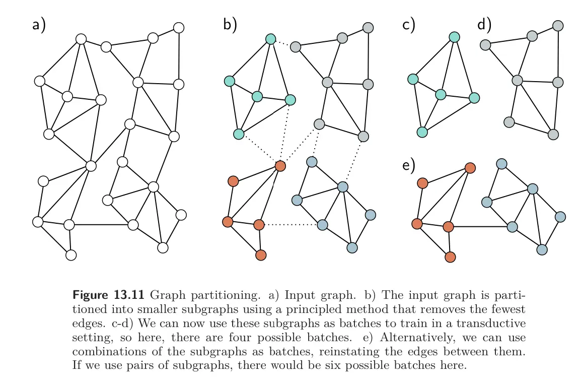
A second way is to cluster the original graph into disjoint subsets of nodes – smaller graphs that are not connected to one another. There are standard algorithms to choose these subsets to maximize the number of internal links while minimizing the number of removed links. These smaller graphs can be treated as batches, or a random subset of them can be combined to form a batch, reinstating any edges between them from the original graph.
Training and Inference
After forming batches using one of the methods above, we can train the network in the same way as for the inductive setting, dividing the nodes into train, test, and validation sets. We’ve essentially converted a transductive problem into an inductive one.
To perform inference, we compute predictions for the unknown nodes based on their k-hop neighborhood. Unlike training, this does not require storing intermediate representations, so it is much more memory efficient.