Graph Convolutional Network

Spatial-based convolutional graph neural networks, or GCNs for short, are a common type of graph neural network.

• They are convolutional in that they update each node by aggregating information from nearby nodes. As such, they induce a relational inductive bias, prioritizing information from neighbors.
• They are spatial-based because they use the original graph structure. This contrasts with spectral-based methods, which apply convolutions in the Fourier domain.

Each layer of the GCN is a function $\mathbf{F}[\bullet ]$ with parameters $\varphi$ that takes the node embeddings and adjacency matrix and outputs new node embeddings. The network can hence be written as:

$$\begin{array}{rl}{\mathbf{H}}_1& =\mathbf{F}[\mathbf{X},\mathbf{A},{\varphi }_0]\\ {\mathbf{H}}_2& =\mathbf{F}[{\mathbf{H}}_1,\mathbf{A},{\varphi }_1]\\ {\mathbf{H}}_3& =\mathbf{F}[{\mathbf{H}}_1,\mathbf{A},{\varphi }_2]\\ ⋮& =⋮\\ {\mathbf{H}}_K& =\mathbf{F}[{\mathbf{H}}_{K-1},\mathbf{A},{\varphi }_{K-1}]\end{array}$$

where $\mathbf{X}$ is the input, $\mathbf{A}$ is the adjacency matrix, ${\mathbf{H}}_k$ contains the modified node embeddings at the $k$-th layer, and ${\varphi }_k$ denotes the parameters that map from layer $k$ to $k+1$.

Design considerations

To design a GCN layer, we want to ensure that it is well-suited to processing graph data (equivarian/invariant to permutations), as well as parameter-efficient.

Equivariance and invariance

Recall that a graph representation is permutation-invariant; any permutation of the node indices does not change the graph. Thus, our model needs to respect this property; each layer must be equivariant with respect to permutations of node incides. In other words, if we permute the node indices, the node embeddings at each stage will be permuted in the same way. Mathematically, if $\mathbf{P}$ is a permutation matrix, we must have:

$${\mathbf{H}}_{k+1}\mathbf{P}=\mathbf{F}[{\mathbf{H}}_k\mathbf{P},{\mathbf{P}}^T\mathbf{AP},{\varphi }_k]$$

For node classification and edge prediction tasks, the output should also be equivariant with respect to permutations of the node indices. However, for graph-level tasks, the final layer aggregates information from across the graph, so the output is invariant to the node order. Recall that the output layer for graph-level classification is:

$$\text{Pr}(y=1|\mathbf{X},\mathbf{A})=\text{sig}[{\beta }_K+{\omega }_K{\mathbf{H}}_{k}1/N]$$

This output layer in fact already achieves invariance, because

$$y=\text{sig}[{\beta }_K+{\omega }_K{\mathbf{H}}_{K}1/N]=\text{sig}[{\beta }_K+{\omega }_K{\mathbf{H}}_{K}P1/N]$$

for any permutation matrix $\mathbf{P}$.

This mirrors the case for images, where segmentation should be equivariant to geometric transformations and classification should be invariant. For images, convolutional and pooling layers partially achieve this with respect to translations, but there is no way to guarantee these properties exactly for more generally transformations. However, for graphs, we can define networks that ensure equivariance or invariance to permutations.

Parameter sharing

Like image processing, graphs benefit from shared convolutional parameters, which is more parameter-efficient than fully connected networks that need to learn how to handle every position separately. We could learn a model with separate parameters at each node, but the network must then independently learn the meaning of the connections in the graph at each position, and training would require many graphs with the same topology. Instead, we build a model that uses the same parameters at every node, reducing the number of parameters and sharing what the network learns at each node across the entire graph.

Recall that a convolution updates a variable by taking a weighted sum of information from its neighbors. One way to think of this is that each neighbor sends a message to the variable of interest, which aggregates these messages to form the update. In images, the neighbors were pixels from a square region around the current position, so the spatial positions are the same. However, in a graph, each node may have a different number of neighbors, and there are no consistent relationships; there is no sense that we can weight information from “above” or “left” of the node differently than from “below” or “right”.

Basic GCN layer

The above considerations lead to a simple GCN layer.

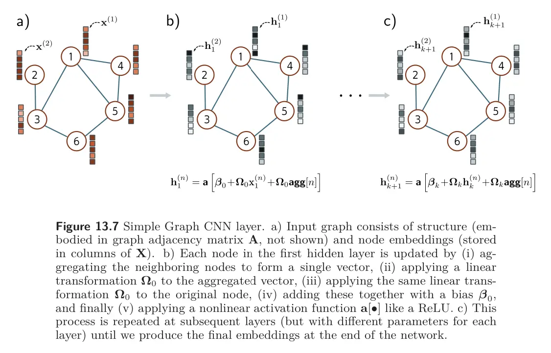
At each node $n$ in layer $k$, we aggregate information from neighboring nodes by summing their node embeddings ${\mathbf{h}}_{\bullet }$:

$$\text{agg}[n,k]=\sum _{m\in \text{ne}[n]}{\mathbf{h}}_k^{(m)}$$

where $\text{ne}[n]$ returns the set of indices of the neighbors of node $n$. Then we apply a linear transformation ${\Omega }_k$ to the embedding ${\mathbf{h}}_k^{(n)}$ at the current node and to its aggregated value, add a bias term ${\beta }_k$, and pass the result through a nonlinear activation function $\mathbf{a}[\bullet ]$, which is applied independently to every member of its vector argument:

$${\mathbf{h}}_{k+1}^{(n)}=a[{\beta }_k+{\Omega }_k\cdot {\mathbf{h}}_k^{(n)}+{\Omega }_k\cdot \text{agg}[n,k]]$$

We can write this more succinctly by noting that the post-multiplication of a matrix by a vector returns a weighted sum of its columns. The $n$-th column of the adjacency matrix $\mathbf{A}$ contains ones at the positions of the neighbors. Hence, if we collect the node embeddings into a $D\times N$ matrix ${\mathbf{H}}_k$ and post-multiply by the adjacency matrix $\mathbf{A}$, the $n$-th column is $\text{agg}[n,k]$. Thus, the update for the nodes is now:

$$\begin{array}{rl}{\text{H}}_{k+1}& =a[{\beta }_k{1}^T+{\Omega }_k{\mathbf{H}}_k+{\Omega }_k{\mathbf{H}}_k\mathbf{A}]\\ & =a[{\beta }_k{1}^T+{\Omega }_k{\mathbf{H}}_k(\mathbf{A}+\mathbf{I})]\end{array}$$

where $1$ is an $N\times 1$ vector containing ones. Here, the nonlinear activation function $\mathbf{a}[\bullet ]$ is applied independently to every member of its matrix argument.

This layer satisfies the design considerations; it’s equivariant to permutations of the node indices, can cope with any number of neighbors, exploits graph structure to provide a relative inductive bias, and shares parameters throughout the graph. We can see it being applied to graph classification.

Variations

Above, we combined messages from adjacent nodes by summing them together with the transformed current node. This was done by computing $\mathbf{H}(\mathbf{A}+\mathbf{I})$. We now consider different approaches to both the combination of the current embedding with the aggregated neighbors, and the aggregation process itself.

Combining current node with aggregated neighbors

The original combination of aggregated neighbors $\mathbf{HA}$ with the current nodes $\mathbf{H}$ was done by just summing them:

$${\text{H}}_{k+1}=a[{\beta }_k{1}^T+{\Omega }_k{\mathbf{H}}_k(\mathbf{A}+\mathbf{I})]$$

Another variation is to multiply the current node by a factor of $(1+{ϵ}_k)$ before contributing to the sum, where ${ϵ}_k$ is a learned scalar that is different for each layer:

$${\mathbf{H}}_{k+1}=a[{\beta }_k{1}^T+{\Omega }_k{\mathbf{H}}_k(\mathbf{A}+(1+{ϵ}_k)\mathbf{I})]$$

This is known as diagonal enhancement.

A related variation applies a different linear transform ${\Psi }_k$ to the current node:

$$\begin{array}{rl}{\mathbf{H}}_{k+1}& =a[{\beta }_k{1}^T+{\Omega }_k{\mathbf{H}}_k\mathbf{A}+{\Psi }_k{\mathbf{H}}_k]\\ & =a\left[{\beta }_k{1}^T+\left[\begin{array}{cc}{\Omega }_k& {\Psi }_k\end{array}\right]\left[\begin{array}{c}{\mathbf{H}}_k\mathbf{A}\\ {\mathbf{H}}_k\end{array}\right]\right]\\ & =a\left[{\beta }_k{1}^T+{\Omega }_k^{\prime }\left[\begin{array}{c}{\mathbf{H}}_k\mathbf{A}\\ {\mathbf{H}}_k\end{array}\right]\right]\end{array}$$

Residual connections

With residual connections, the aggregated representation from the neighbors is transformed and passed through the activation function before summation or concatenation with the current node. For the latter case, the associated equations are:

$${\mathbf{H}}_{k+1}=\left[\begin{array}{c}a[{\beta }_k{1}^T+{\Omega }_k{\mathbf{H}}_k\mathbf{A}]\\ {\mathbf{H}}_k\end{array}\right]$$

Mean aggregation

The above methods aggregate the neighbors by summing the node embeddings. However, it’s possible to combine the embeddings in different ways. Sometimes it’s better to take the average of the neighbors rather than the sum; this can be superior if the embedding information is more important and the structural information less so since the magnitude of the neighborhood contributions will not depend on the number of neighbors:

$$\text{agg}[n]=\frac{1}{\left|\text{ne}\right|[n]}\sum _{m\in \text{ne}[n]}{\mathbf{h}}_m$$

where as before, $\text{ne}[n]$ denotes a set containing the indices of the neighbors of the $n$-th node. The above equation can be computed neatly in matrix form by introducing the diagonal $N\times N$ matrix $\mathbf{D}$. Each non-zero element of this matrix contains the number of neighbors for the associated node. It follows that each diagonal element in the inverse matrix ${\mathbf{D}}^{-1}$ contains the denominator that we need to compute the average. The new GCN layer can be written as:

$${\mathbf{H}}_{k+1}=a[{\beta }_k{1}^T+{\Omega }_k{\mathbf{H}}_k({\mathbf{AD}}^{-1}+\mathbf{I})]$$

Kipf Normalization

There are many variations of graph neural networks based on mean aggregation. Sometimes the current node is included with its neighbors in the mean computation rather than treated separately. In Kipf normalization, the sum of the node representations is normalized as:

$$\text{agg}[n]=\sum _{m\in \text{ne}[n]}\frac{{\mathbf{h}}_m}{\sqrt{\left|\text{ne}[n]\right|\left|\text{ne}[m]\right|}}$$

with the logic that information coming from nodes with a very large number of neighbors should be down-weighted since there are many connections and they provide less unique information. This can also be expressed in matrix form using the degree matrix:

$${\mathbf{H}}_{k+1}=a[{\beta }_k{1}^T+{\Omega }_k{\mathbf{H}}_k({\mathbf{D}}^{-1/2}\mathbf{A}{\mathbf{D}}^{-1/2}+\mathbf{I})]$$

Max pooling aggregation

An alternative operation that is also invariant to permutation is computing the maximum of a set of objects. The max pooling aggregation operator is:

$$\text{agg}[n]=\underset{m\in \text{ne}[n]}{\max }[{\mathbf{h}}_m]$$

where the operator $\text{max}[\bullet ]$ return the element-wise maximum of the vectors ${\mathbf{h}}_m$ that are neighbors to the current node $n$.

dl
Graph convolutional networks::Take the node embeddings and adjacency matrix and outputs new node embeddings, aggregating information from nearby nodes.