Backpropagation Toy Example

Consider a model $f[x,\varphi ]$ with eight scalar parameters $\varphi =\{{\beta }_0,{\omega }_0,{\beta }_1,{\omega }_1,{\beta }_2,{\omega }_2,{\beta }_3,{\omega }_3\}$ that consists of a composition of functions $\sin [\bullet ],\exp [\bullet ]$ and $\cos [\bullet ]$:

$$f[x,\varphi ]={\beta }_3+{\omega }_3\cdot \cos [{\beta }_2+{\omega }_2\cdot \exp [{\beta }_1+{\omega }_1\cdot \sin [{\beta }_0+{\omega }_0\cdot x]]]$$

and a least squares loss function $L[\varphi ]={\sum }_i{\ell }_i$ with individual terms:

$${\ell }_i=(f[x_i,\varphi ]-y_i{)}^2$$

where $x_i$ is the $i$-th training input, and $y_i$ is the $i$-th training output. You can think of this as a simple neural network with one input, one output, one hidden unit at each layer, and different activation functions $\sin [\bullet ],\exp [\bullet ]$ and $\cos [\bullet ]$ between each layer.

We aim to compute the derivatives of ${\ell }_i$ with respect to each of the eight parameters:

$$\frac{\partial {\ell }_i}{\partial {\beta }_0},\frac{\partial {\ell }_i}{\partial {\omega }_0},\frac{\partial {\ell }_i}{\partial {\beta }_1},\frac{\partial {\ell }_i}{\partial {\omega }_1},\frac{\partial {\ell }_i}{\partial {\beta }_2},\frac{\partial {\ell }_i}{\partial {\omega }_2},\frac{\partial {\ell }_i}{\partial {\beta }_3},\frac{\partial {\ell }_i}{\partial {\omega }_3}$$

Of course, we could find expressions for these derivatives by hand and compute them directly. However, some of these expressions are quite complex. Such expressions are awkward to derive and code without mistakes and do not exploit the inherent redundancy.

Backpropagation is an efficient method for computing all of these derivatives at once. It consists of a forward pass, in which we compute and store a series of intermediate values and the network output, and a backward pass, in which we calculate the derivatives of each parameter, starting at the end of the network, and re-use previous calculations as we move toward the start.

Forward Pass

We treat the computation of the loss as a series of calculations:

$$\begin{array}{rl}{f}_0& ={\beta }_0+{\omega }_0\cdot x_i\\ h_1& =\sin [f_0]\\ f_1& ={\beta }_1+{\omega }_1\cdot h_1\\ h_2& =\exp [f_1]\\ f_2& ={\beta }_2+{\omega }_2\cdot h_2\\ h_3& =\cos [f_2]\\ f_3& ={\beta }_3+{\omega }_3\cdot h_3\\ {\ell }_i& =(f_3-y_i{)}^2\end{array}$$

We compute and store the values of the intermediate variables $f_k$ and $h_k$.

Backward pass 1

We now compute the derivatives of ${\ell }_1$ with respect to these intermediate variables, but in reverse order.

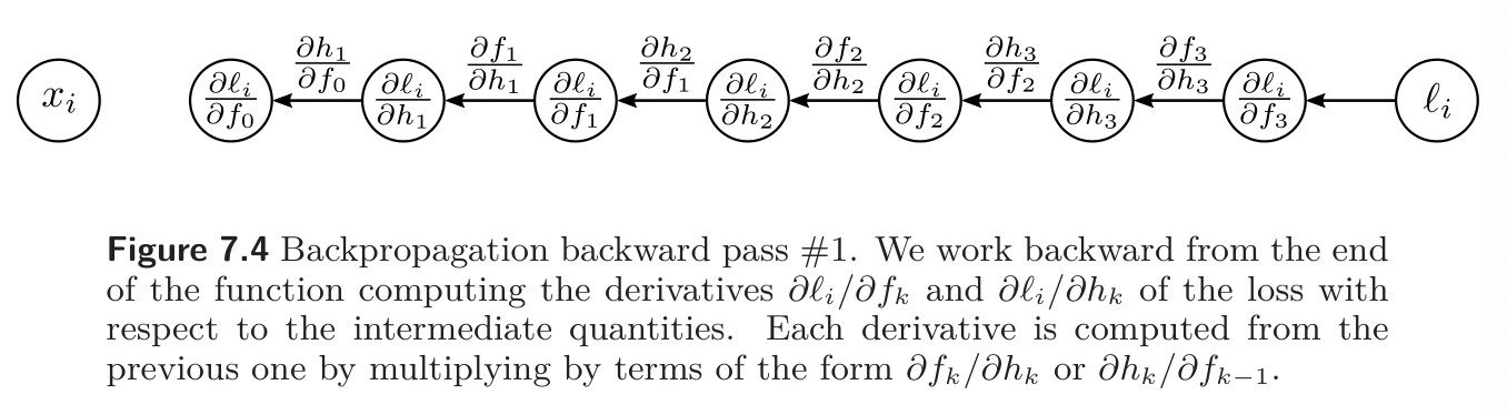
The first one is very straightforward:

$$\frac{\partial {\ell }_i}{\partial f_3}=2(f_3-y_i)$$

The next derivative can be calculated using the chain rule:

$$\frac{\partial {\ell }_i}{\partial h_3}=\frac{\partial {\ell }_i}{\partial f_3}\frac{\partial f_3}{\partial h_3}$$

• The left side asks how ${\ell }_i$ changes when $h_3$ changes
• The right side says we can decompose this into (i) how ${\ell }_i$ changes when $f_3$ changes and (ii) how $f_3$ changes when $h_3$ changes. In the original equations, $h_3$ changes $f_3$, which changes ${\ell }_i$, and the derivatives represent the effects of this chain. Notice that we already computed the first derivative and the other is just the derivative of ${\beta }_3+{\omega }_3\cdot h_3$ with respect to $h_3$.

We can continue this way:

$$\begin{array}{rl}\frac{\partial {\ell }_i}{\partial f_2}& =\left(\frac{\partial {\ell }_i}{\partial f_3}\frac{\partial f_3}{\partial h_3}\right)\frac{\partial h_3}{\partial f_2}\\ \frac{\partial {\ell }_i}{\partial h_2}& =\left(\frac{\partial {\ell }_i}{\partial f_3}\frac{\partial f_3}{\partial h_3}\frac{\partial h_3}{\partial f_2}\right)\frac{\partial f_2}{\partial h_2}\\ \frac{\partial {\ell }_i}{\partial f_1}& =\left(\frac{\partial {\ell }_i}{\partial f_3}\frac{\partial f_3}{\partial h_3}\frac{\partial h_3}{\partial f_2}\frac{\partial f_2}{\partial h_2}\right)\frac{\partial h_2}{\partial f_1}\\ \frac{\partial {\ell }_i}{\partial h_1}& =\left(\frac{\partial {\ell }_i}{\partial f_3}\frac{\partial f_3}{\partial h_3}\frac{\partial h_3}{\partial f_2}\frac{\partial f_2}{\partial h_2}\frac{\partial h_2}{\partial f_1}\right)\frac{\partial f_1}{\partial h_1}\\ \frac{\partial {\ell }_i}{\partial f_0}& =\left(\frac{\partial {\ell }_i}{\partial f_3}\frac{\partial f_3}{\partial h_3}\frac{\partial h_3}{\partial f_2}\frac{\partial f_2}{\partial h_2}\frac{\partial h_2}{\partial f_1}\frac{\partial f_1}{\partial h_1}\right)\frac{\partial h_1}{\partial f_0}\end{array}$$

In each case, we already calculated the quantities in the brackets in the previous step, and the last term has a simple expression. These equations embody Observation 2 we made in Backpropagation Intuition; we can reuse the previously computed derivatives if we calculate them in reverse order.

Backward pass 2

Finally, we consider how the loss ${\ell }_i$ changes when we change the parameters $\{{\beta }_k\}$ and $\{{\omega }_k\}$.

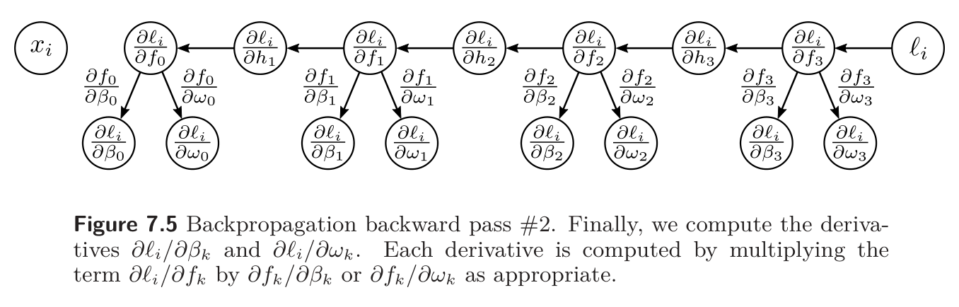
Once again, we apply the chain rule:

$$\begin{array}{rl}\frac{\partial {\ell }_i}{\partial {\beta }_k}& =\frac{\partial {\ell }_i}{\partial f_k}\frac{\partial f_k}{\partial {\beta }_k}\\ \frac{\partial {\ell }_i}{\partial {\omega }_k}& =\frac{\partial {\ell }_i}{\partial f_k}\frac{\partial f_k}{\partial {\omega }_k}\end{array}$$

In each case, the first term on the right side was already computed above. When $k>0$, we have $f_k$ = ${\beta }_k+{\omega }_k\cdot h_k$, so

$$\frac{\partial f_k}{\partial {\beta }_k}=1\text{and}\frac{\partial f_k}{\partial {\omega }_k}=h_k$$

This is consistent with Observation 1 from Backpropagation Intuition; the effect of a change in the weight ${\omega }_k$ is proportional to the value of the source $h_k$ which was stored in the forward pass. The final derivatives from the term $f_0={\beta }_0+{\omega }_0\cdot x_i$ are:

$$\frac{\partial f_0}{\partial {\beta }_0}=1\text{and}\frac{\partial f_0}{\partial {\omega }_0}=x_i$$

Backpropagation is both simpler and more efficient than computing the derivatives individually.