Loss functions in the case of gradient descent for linear regression always have a single well-defined global minimum. They are convex, such that every chord (line segment between two points on the surface) lies above the function and does not intersect it. Convexity implies that whenever we initialize the parameters, we are bound to reach the minimum if we keep walking downhill; the training procedure can’t fail.
In practice, loss functions for most nonlinear models, including both shallow neural networks and deep neural networks, are non-convex. Visualizing neural network loss functions is challenging due to the number of parameters. Hence, we first explore a simpler nonlinear model with two parameters to gain properties of non-convex loss functions:
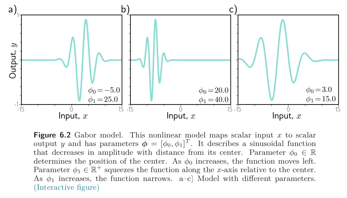
This Gabor model maps scalar input to scalar output and consists of a sinusoidal component (creating an oscillatory function) multiplied by a negative exponential component (causing the amplitude to decrease as we move from the center). It has two parameters , where determines the mean position of the function and stretches or squeezes it along the -axis.
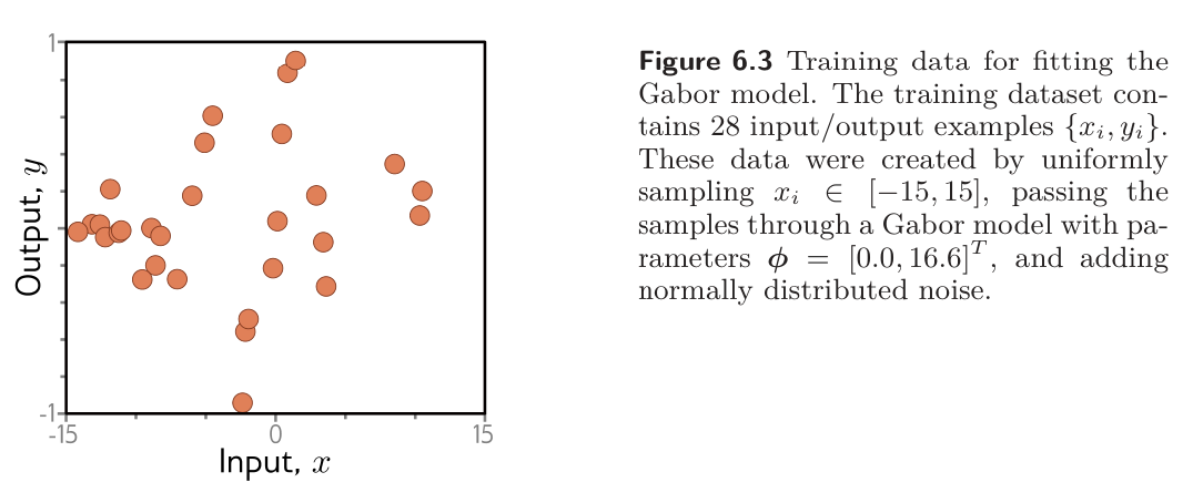
Consider a training set of examples . The least squares loss function for training examples is defined as:
The goal is to find the parameters that minimize this loss.
Local Minima & Saddle Points
The figure below shows the loss function associated with the Gabor model for this dataset. There are numerous local minima (cyan circles); the gradient is zero, and the loss increases if we move in any direction, but we are not at the global minimum (gray circle).
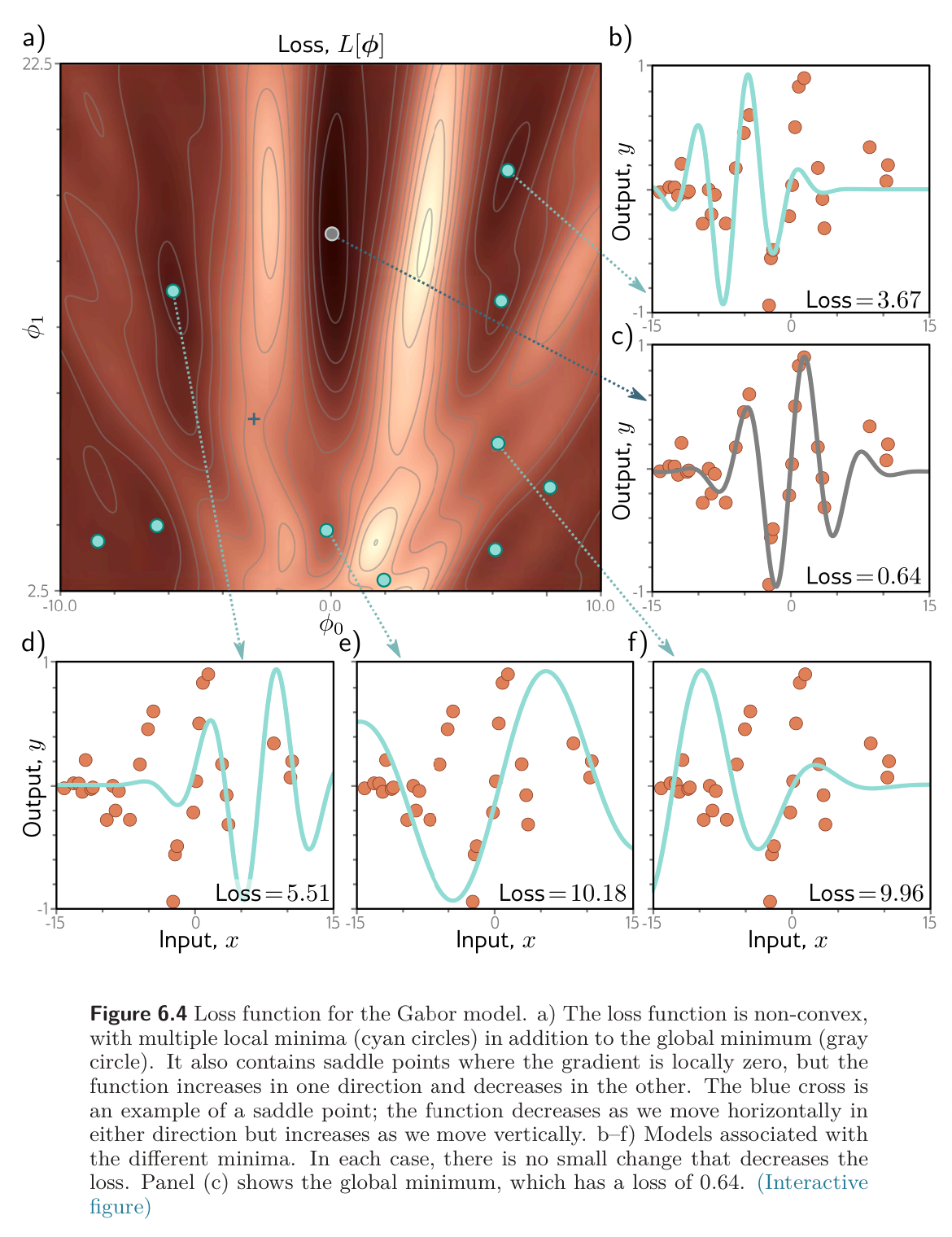
If we start in a random position and use gradient descent to go downhill, there’s no guarantee that we’ll wind up at the global minimum and find the best parameters. It’s equally or even more likely that the algorithm will terminate in one of the local minima. There’s also no way of knowing whether there’s a better solution elsewhere.
The loss function also contains saddle points (blue cross). Here, the gradient is zero, but the function increases in some directions and decreases in other. If the current parameters are not exactly at the saddle point, then gradient descent can escape by moving downhill. However, the surface near the saddle point is flat, so it’s hard to be sure that training hasn’t converged; if we terminate the algorithm when the gradient is small, we may erroneously stop near a saddle point.