Damped Response for Second-Order System

For a damped system, we have

$$m\ddot{x}+c\dot{x}+kx=f(t)$$

Like the undamped case, we aim to solve the characteristic equation to determine the response of the system. We have

$$\begin{array}{rl}m{s}^2+cs+k& =0\\ s^2+\frac{c}{m}s+\frac{k}{m}& =0\end{array}$$

Recall that $\sqrt{k/m}={\omega }_n$, so $k/m={\omega }_n^2$. Let:

$$\begin{array}{rl}\frac{c}{m}& =2\zeta {\omega }_n\\ \zeta & =\frac{c}{2m{\omega }_n}=\frac{c}{c_{\text{cr}}}\end{array}$$

We can then say:

$$c_{\text{cr}}=2m{\omega }_n=2m\sqrt{\frac{k}{m}}=2\sqrt{km}$$

and

$$\zeta =\frac{c}{2\sqrt{km}}$$

where $\zeta$ is called the damping ratio. Then, we have

$$\begin{array}{rl}{s}^2+\frac{c}{m}s+\frac{k}{m}& =0\\ s^2+2\zeta {\omega }_n+{\omega }_n^2& =0\\ s& =\frac{-2\zeta {\omega }_n\pm \sqrt{4{\zeta }^2{\omega }_n^2-4{\omega }_n^2}}{2}\\ & =-\zeta {\omega }_n\pm {\omega }_n\sqrt{{\zeta }^2-1}\end{array}$$

Recall that in general, for second-order systems we have:

$$X(s)=\underset{\text{ZSR}}{\underbrace{\frac{F(s)}{m{s}^2+cs+k}}}+\underset{\text{ZIR}}{\underbrace{\frac{msx(0)+m\dot{x}(0)+cx(0)}{m{s}^2+cs+k}}}$$

The free damped response, where $F(s)=0$, would then be

$$\begin{array}{rl}X(s)& =\frac{msx(0)+m\dot{x}(0)+cx(0)}{m{s}^2+cs+k}\\ & =\frac{sx(0)+\dot{x}(0)+\frac{c}{m}x(0)}{s^2+2\zeta {\omega }_n+{\omega }_n^2}\end{array}$$

The poles are at

$$s=-\zeta {\omega }_n\pm {\omega }_n\sqrt{{\zeta }^2-1}$$

There are three cases we need to consider.

Case 1: Overdamped

This occurs when $\zeta >1$ (or equivalently $c/c_{\text{cr}}>1$). We have

$$\zeta =\frac{c}{c_{\text{cr}}}=\frac{c}{2m{\omega }_n}=\frac{c}{2\sqrt{km}}$$

If we have $\zeta >1$, that means have have $c>\sqrt{2km}$.

Since $\zeta >1$, we have $\sqrt{{\zeta }^2-1}>0$, which means that $s=-\zeta {\omega }_n\pm {\omega }_n\sqrt{{\zeta }^2-1}$ produces two distinct real poles. Thus, we have

$$\begin{array}{r}{s}_1=-\zeta {\omega }_n-{\omega }_n\sqrt{{\zeta }^2-1}\\ s_2=-\zeta {\omega }_n+{\omega }_n\sqrt{{\zeta }^2-1}\end{array}$$

Simplifying:

$$\begin{array}{rl}{s}_1& ={\omega }_n(-\zeta -\sqrt{{\zeta }^2-1})\\ s_2& ={\omega }_n(-\zeta +\sqrt{{\zeta }^2-1})\end{array}$$

where $s_1<s_2$ or $-s_1>-s_2$.

This gives:

$$X(s)=\frac{sx(0)+\dot{x}(0)+2\zeta {\omega }_{n}x(0)}{(s-s_1)(s-s_2)}$$

Converting back to time domain:

$$x(t)=C_1{e}^{s_{1}t}+C_2{e}^{s_{2}t}$$

If we let $\tau =-\frac{1}{s_1}$ and ${\tau }_2=-\frac{1}{s_2}$, this can be written as

$$x(t)=C_1{e}^{-t/{\tau }_1}+C_2{e}^{-t/{\tau }_2}$$

Note that since $s_2>s_1$, we call $s_2$ the dominant pole.

Overdamped Example

Let’s say we have have:

• $\zeta =\sqrt{10}\approx 3.2$
• ${\omega }_n=100\frac{\text{rad}}{s}$ Then, we have:

$$\begin{array}{r}{s}_1=-100(\sqrt{10}-\sqrt{10-1})=-20\\ s_2=-100({\sqrt{10}}_{\sqrt{10-1}})=-620\end{array}$$

So:

$$\begin{array}{rlr}x(t)& =C_1{e}^{s_{1}t}+C_2{e}^{s_{2}t}=C_1{e}^{-20t}+C_2{e}^{-620t}& =C_1{e}^{\frac{-t}{1/20}}+C_2{e}^{\frac{-t}{1/620}}\end{array}$$

where ${\tau }_1=\frac{1}{20}=50\text{ ms}$ and ${\tau }_2=\frac{1}{620}=1.2\text{ ms}$

Case 2: Critically Damped

In the critically damped cause $\zeta =1$, or $\frac{c}{c_{\text{cr}}}=1$, such that $c=c_{\text{cr}}=2\sqrt{km}$. This is the minimum damping to have no oscillation.

In this case, we have ${\zeta }^2-1=0$, so $s=-\zeta {\omega }_n\pm 0$, so we have repeated real poles, $s=-{\omega }_n$. Thus, we have:

$$\begin{array}{rl}{s}^2+2\zeta {\omega }_{n}s+{\omega }_n^2& =s^2+{\omega }_{n}s+{\omega }_n^2\\ & =[s-(-{\omega }_n){]}^2\end{array}$$

This gives:

$$\begin{array}{rl}X(s)& =\frac{sx(0)+2\zeta {\omega }_{n}s+{\omega }_n^2}{(s+{\omega }_n{)}^2}\\ x(t)& =(C_1+t{C}_2)e^{st}=(C_1+t{C}_2)e^{-{\omega }_{n}t}\end{array}$$

Case 3: Underdamped

For the underdamped case, we have $0<\zeta <1$, such that $c<c_{\text{cr}}$ or $c<2\sqrt{km}$. Then, we have

$$s=-\zeta {\omega }_n\pm \omega \sqrt{{\zeta }^2-1}$$

where

$$\sqrt{{\zeta }^2-1}=\sqrt{(-1)(1-\zeta {)}^2}=j\sqrt{1-{\zeta }^2}$$

Thus, we have

$$s=-\zeta {\omega }_n\pm j\underset{{\omega }_d}{\underbrace{{\omega }_n\sqrt{1-{\zeta }^2}}}$$

where ${\omega }_d={\omega }_n\sqrt{1-{\zeta }^2}$ is the damped natural frequency. Then, we can write $s$ as

$$s=-\zeta {\omega }_n\pm j{\omega }_d$$

and

$$\begin{array}{rl}{e}^{st}& =e^{-(\zeta {\omega }_n\pm j{\omega }_d)t}\\ & =e^{-\zeta {\omega }_n}[\cos {\omega }_{d}t\pm j\sin {\omega }_{d}t]\end{array}$$

This damped oscillation plot looks something like:

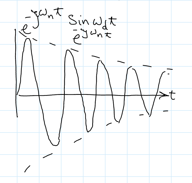
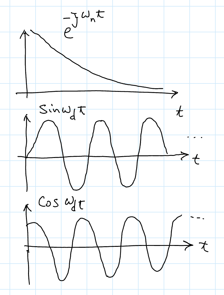
Essentially, the amplitude of oscillation follows $e^{-\zeta {\omega }_{n}t}$.

For underdamped systems, the time constant is

$$\tau =\frac{1}{\zeta {\omega }_n}=\frac{2m}{c}$$

so we have:

$$e^{st}=e^{-t/\tau }[\cos ({\omega }_{d}t)\pm j\sin ({\omega }_{d}t)]$$

In the time domain, this can be written as

$$\begin{array}{rl}x(t)& =C_1{e}^{s_{1}t}+C_2{e}^{s_{2}t}\\ & =e^{-t/\tau }[C_1{e}^{\text{Im}(s_1)t}+C_2{e}^{\text{Im}(s_2)t}]\end{array}$$

Alternatively, we can write

$$x(t)=e^{-\zeta {\omega }_{n}t}[A\sin ({\omega }_{d}t)+x(0)\cos ({\omega }_{d}t)]$$

such that

$$A=\frac{\zeta }{\sqrt{1-{\zeta }^2}}x(0)+\frac{1}{{\omega }_d}\dot{x}(0)$$

and

$$x(t)=D{e}^{-\zeta {\omega }_{n}t}\sin ({\omega }_{d}t+\varphi )$$

Graphical Interpretation

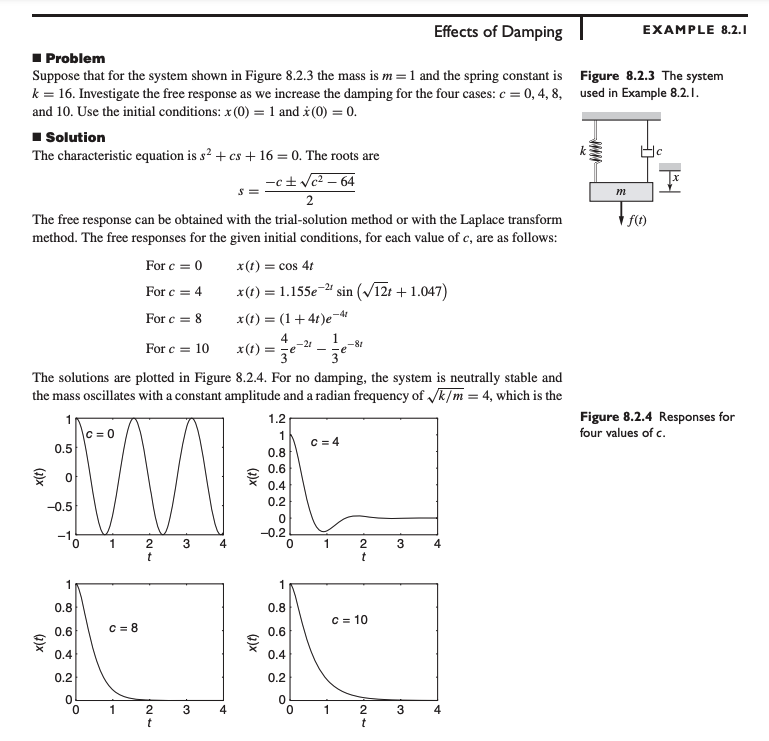
Effects of Damping

With $c<c_{\text{cr}}$, oscillation will occur. This is illustrated in the example problem below.

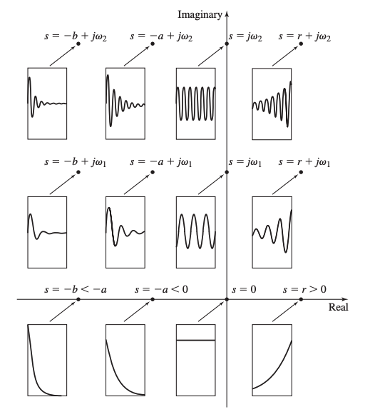
Effect of Root Location

In finding the roots of the characteristic equation in the complex plane, the location of the roots affects the free response. The real part of the root is plotted on the horizontal axis, and the imaginary part is plotted on the vertical axis. Because the roots are conjugates of each other, we only show the upper root.

• Unstable behavior occurs if any root lies to the right of the imaginary axis.
• The response oscillates only when a root has a nonzero imaginary part.
• The greater the imaginary part, the higher the frequency of oscillation.
• The farther to the left the root lies, the faster the response due to that root decays.