Elliptic Equations

Elliptic equations represent steady state problems, such as temperature distribution in plate or rod, after sufficient time elapses to achieve steady state.

Heated Plate Example

The Laplace’s Equation is used here:

$$\frac{{\partial }^{2}T}{\partial x^2}+\frac{{\partial }^{2}T}{\partial y^2}=0$$

Consider a thin plate (thickness $\Delta z$) insulated on the front and back surfaces. A small element of width $\Delta x$ and $\Delta y$ can be described at steady state by heat flux into and out of the element:

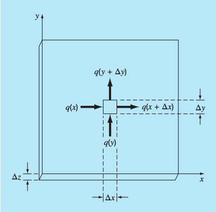
At steady state, the flow of heat into the element over a unit time period $\Delta t$ must equal the flow out, as in

$$q(x)\Delta y\Delta z\Delta t+q(y)\Delta x\Delta z\Delta t=q(x+\Delta x)\Delta y\Delta z\Delta z\Delta t+q(y+\Delta y)\Delta x\Delta z\Delta t$$

where $q$ represents heat flux.

Dividing by $\Delta z$ and $\Delta t$ and collecting terms yields:

$$[q(x)-q(x+\Delta x)\Delta y]+[q(y)+q(y+\Delta y)]\Delta x=0$$

Multiplying the first term by $\Delta x/\Delta x$ and the second by $\Delta y/\Delta y$ gives:

$$\frac{q(x)-q(x+\Delta x)}{\Delta x}\Delta x\Delta y+\frac{q(y)-q(y+\Delta y)}{\Delta y}\Delta y\Delta x=0$$

Dividing by $\Delta x\Delta y$ and taking the limit results in

$$-\frac{\partial q}{\partial x}-\frac{\partial q}{\partial y}=0$$

The relationship between flux and temperature is given by Fourier’s law of heat conduction:

$$q_i=-k\rho C\frac{\partial T}{\partial i}$$

where the temperature $T$ is defined as:

$$T=\frac{H}{\rho CV}$$

The term $k\rho C$ is sometimes written as a coefficient of thermal conductivity, $k^{\prime }$.

Substituting $q_i=-k\rho C\frac{\partial T}{\partial i}$ into $-\frac{\partial q}{\partial x}-\frac{\partial q}{\partial y}=0$ gives:

$$\frac{{\partial }^{2}T}{\partial x^2}+\frac{\partial T^2}{\partial y^2}=0$$

which is just the Laplace equation.

Solution

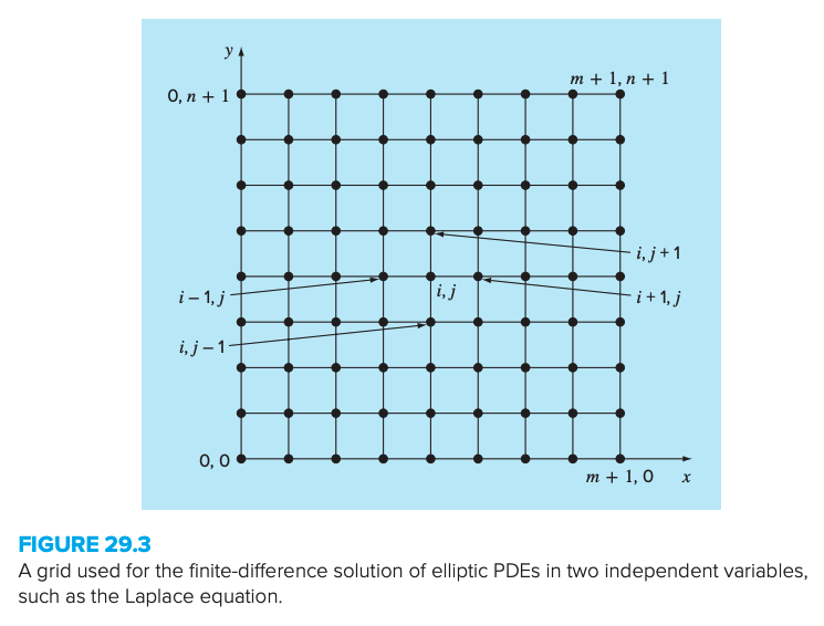
To solve problems like these, numerical methods based on finite differences representations are used. These are based on treating the plate as a grid of discrete points.

Central differences based on the grid scheme are:

$$\frac{{\partial }^{2}T}{\partial x^2}=\frac{T_{i+1,j}-2T_{i,j}+T_{i-1,j}}{\Delta x^2}$$

and

$$\frac{\partial T^2}{\partial y^2}=\frac{T_{i,j+1}-2T_{i,j}+T_{i-1,j}}{\Delta y^2}$$

which have errors of $O[\Delta (x{)}^2]$ and $O[\Delta (y{)}^2]$. Substituting these expressions give:

$$\frac{T_{i+1,j}-2T_{i,j}+T_{i-1,j}}{\Delta x^2}+\frac{T_{i,j+1}-2T_{i,j}+T_{i-1,j}}{\Delta y^2}=0$$

For the square grid, $\Delta x=\Delta y$, and by collection of terms, we have:

$$T_{i+1,j}+T_{i-1,j}+T_{i,j+1}+T_{i,j-1}-4T_{i,j}=0$$

This relationship holds for all interior points on the plate and is referred to as the Laplacian difference equation.

Important: Boundary conditions along the edges of the plate must be specified to obtain a unique solution. The simplest case is where the temperature at the boundary is set at a fixed value (Dirichlet boundary condition):

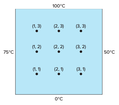
For example, let’s consider grid point $(1,1)$:

$$T_{21}+T_{01}+T_{12}+T_{10}-4T_{11}=0$$

For our problem, $T_{01}=75$ and $T_{10}=0$, so we have:

$$-4T_{11}+T_{12}+T_{12}=75$$

Applying this method at each grid point results in a system of 9 equations and 9 unknowns:

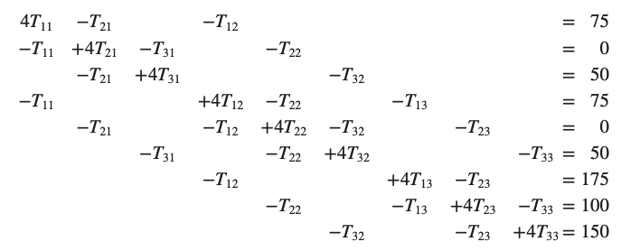
This can be solved using Gauss-Seidel or similar methods.

Secondary variables

Temperature is the primary variable in the heated plate problem because its distribution is described by the Laplace equation. However, we may have secondary variables of interest. For example, a secondary variable for the plate is the rate of heat flux across the plate’s surface. This can be calculated with Fourier’s law, $q_i=-k\rho C\frac{\partial T}{\partial i}$, discussed above.

Centered finite-difference approximations for the first derivatives can be substituted to give the following heat flux values in $x$ and $y$ dimensions:

$$\begin{array}{r}{q}_x=-k^{\prime }\frac{T_{i+1,j}-T_{i-1,j}}{2\Delta x}\\ q_y=-k^{\prime }\frac{T_{i,j+1}-T_{i,j-1}}{2\Delta y}\end{array}$$

The resultant heat flux can be computed from these two quantities using $q_n=\sqrt{q_x^2+q_y^2}$ where the direction of $q_n$ is given by:

$$\begin{array}{rl}\theta & ={\tan }^{-1}\left(\frac{q_y}{q_x}\right),q_x>0\\ \theta & ={\tan }^{-1}\left(\frac{q_y}{q_x}\right)+\pi ,q_x<0\end{array}$$

With this, given some boundary conditions and a heat constant, we can find heat flux values at each point on the grid. For example, if we have $k^{\prime }=0.49\text{ cal / s cm }°,\text{C}$ and the same boundary conditions as above, grid point $(1,1)$ would have:

$$\begin{array}{rl}{q}_x& =(-0.49)\frac{33.29755-75}{2(10)}=1.022\\ q_y& =(-0.49)\frac{63.21152-75}{2(10)}=-1.549\\ q_n& =\sqrt{(1.022{)}^2+(-1.549{)}^2}=1.856\\ \theta & ={\tan }^{-1}\left(\frac{-1.549}{1.022}\right)=-56.584°\end{array}$$

Neumann Boundary Conditions

Instead of constant boundary conditions, they can be based on derivative. For the heated plate specifying the derivative at the boundary is equivalent to specifying the flux $q$ at the boundary.

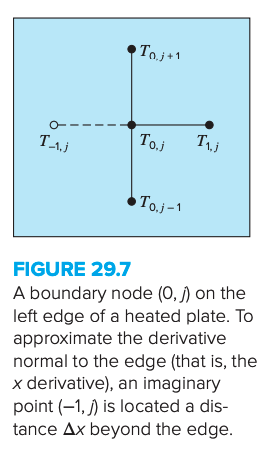
For the point $(0,j)$, we can apply the Laplace equation $T_{i+1,j}+T_{i-1,j}+T_{i,j+1}+T_{i,j-1}-4T_{i,j}=0$ to get:

$$T_{1,j}+T_{-1,j}+T_{0,j+1}+T_{0,j-1}-4T_{0,j}=0$$

Note that an imaginary point $(-1,j)$ lying outside the plate is required for this equation. We can use this point to incorporate the derivative boundary condition into the problem by representing the first derivative in the $x$ dimension at $(0,j)$ by the finite divided difference:

$$\frac{\partial T}{\partial x}\approx \frac{T_{i,j}-T_{-1,j}}{2\Delta x}$$

which ban be solved for:

$$T_{-1,j}=T_{1,j}-2\Delta x\frac{\partial T}{\partial x}$$

Now we have a relationship for $T_{-1,j}$ that actually includes the derivative. It can be substituted to give:

$$2T_{1,j}-2\Delta x\frac{\partial T}{\partial x}+T_{0,j+1}+T_{0,j-1}-4T_{0,j}=0$$

Thus, we have incorporated the derivative into the balance. Similar relationships can be developed for derivative boundary conditions at the other edges.