Parabolic Equations

Parabolic PDEs include a time-dependent component – transient effects up to steady-state response. Let us continue considering the heated plate example introduced in Parabolic Equations. Rather than examine the steady-state case, the present balance also considers the amount of heat stored in the element over a unit time period $\Delta t$.

The balance expression for parabolic equations also considers the amount of heat stored in the element over a unit time period $\Delta t$, such that we have $\text{inputs}-\text{outputs}=\text{storage}$.

$$q(x)\Delta y\Delta z\Delta t-q(x+\Delta x)\Delta y\Delta z\Delta t=\Delta x\Delta y\Delta z\rho C\Delta T$$

Dividing by the volume of the element ($\Delta x\Delta y\Delta z$) and $\Delta t$ gives:

$$\frac{q(x)-q(x+\Delta x)}{\Delta x}=\rho C\frac{\Delta T}{\Delta t}$$

Taking the limit yields

$$-\frac{\partial q}{\partial x}=\rho C\frac{\partial T}{\partial t}$$

We can find an expression for $q$ based on Fourier’s law of heat conduction, we have:

$$q_i=-k\rho C\frac{\partial T}{\partial i}$$

Here $q_i$ is heat flux in the direction of the $i$ dimension, $k$ is the coefficient of thermal conductivity, $\rho$ is the density of the material. $C$ is the heat capacity of the material.

Substituting this into our $\frac{\partial q}{\partial x}$ gives

$$k\frac{{\partial }^{2}T}{\partial x^2}=\frac{\partial T}{\partial t}$$

We are solving the equation with respect to two variables, position $x$ and time $t$.

For position, we can use the same centered finite divided-difference expression that we used in Elliptic Equations:

$$\frac{{\partial }^{2}T}{\partial x^2}=\frac{T_{i+1}^l-2T_i^l+T_{i-1}^l}{\Delta x^2}$$

For time, we can use forward finite divided difference:

$$\frac{\partial T}{\partial x}=\frac{T_i^{l+1}-T_i^l}{\Delta t}$$

Substituting:

$$k\frac{T_{i+1}^l-2T_i^l+T_{i-1}^l}{\Delta x^2}=\frac{T_i^{l+1}-T_i^l}{\Delta t}$$

Solving:

$$T_i^{l+1}=T_i^l+\lambda (T_{i+1}^l-2T_i^l+T_{i-1}^l)$$

where $\lambda =k\Delta t/(\Delta x{)}^2$.

This is applicable to all interior nodes. It then provides an explicit means to compute values at each node for a future time based on the present values at the node and its neighbors.

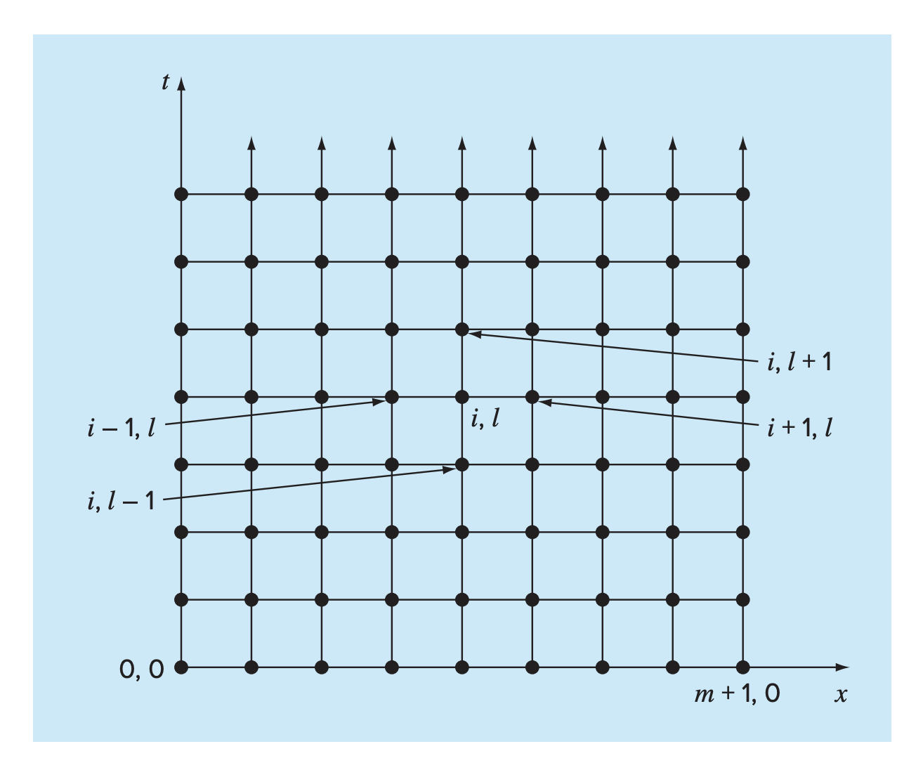
The grid below is used for the finite-difference solution of parabolic PDEs in two independent variables such as the heat-conduction equation. Note that grid is open-ended in time.

Convergence and Stability

• Convergence means that as $\Delta x$ and $\Delta t$ approach zero, the results of the finite-difference technique approach the true solution.
• Stability means that errors at any stage of the computation are not amplified but are attenuated as the computation progresses

Note that finite difference methods propagate the solutions from boundary conditions inwards, so not all points that should affect the solution are included. We can address this through implicit equations, but with added complexity.

Implicit methods to solve PDEs are unconditionally stable, but do incur a penalty for calculation time.

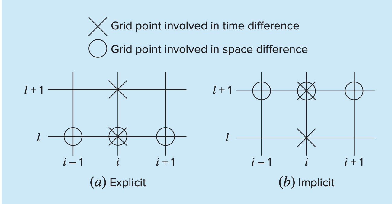
• For explicit methods, we approximate the spatial derivative at time level $l$. Recall above that when we substituted this approximation into the PDE, we obtained a difference equation with a single unknown $T_i^{l+1}$
• For implicit methods, the spatial derivative is approximated, for example something like $\frac{{\partial }^{2}T}{\partial x^2}\approx \frac{T_{i+1}^{l+1}-2T_i^{l+1}+T_{i-1}^{l+1}}{\Delta x^2}$. When this relationship is substituted into the original PDE, the resulting difference equation contains several unknowns. Thus, it cannot be solved explicitly by simple algebraic rearrangement. Instead, the entire system of equations must be solved simultaneously. This is possible because, along with the boundary conditions, the implicit formulations result in a set of linear algebraic equations with the same number of unknowns. Thus, the method reduces to the solution of a set of simultaneous equations at each point in time.

Crank-Nicholson

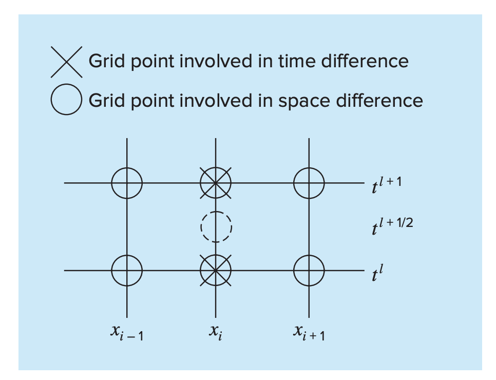
The Crank-Nicolson method provides an alternative implicit scheme that is second-order accurate in both space and time. To provide this accuracy, difference approximations are developed at the midpoint of the time increment. To do this, the temporal first derivative can be approximated at $t_{l+1/2}$ by

$$\frac{\partial T}{\partial t}\approx \frac{T_i^{l+1}-T_i}{\Delta t}$$

The second derivative in space can be determined at the midpoint by averaging the difference approximations at the beginning ($t^l$) and at the end ($t^{l+1}$) of the time increment:

$$\frac{{\partial }^{2}T}{\partial x^2}\approx \frac{1}{2}\left[\frac{T_{i+1}^l-2T_i^l+T_{i+1}^l}{(\Delta x{)}^2}+\frac{T_{i+1}^{l+1}-2T_i^{l+1}+T_{i-1}^{l+1}}{(\Delta x{)}^2}\right]$$

Then, we substitute these into $k\frac{{\partial }^{2}T}{\partial x^2}=\frac{\partial T}{\partial t}$ to solve.