1D Kalman Filter without Process Noise

This shows the derivation of the Kalman Filter in one dimension; the goal is intuition and clarity.

Unlike the alpha-beta-gamma filter, the Kalman filter treats measurements, the current state estimate, and the predicted state estimate as normally distributed random variables. Each random variable is described by its mean and variance.

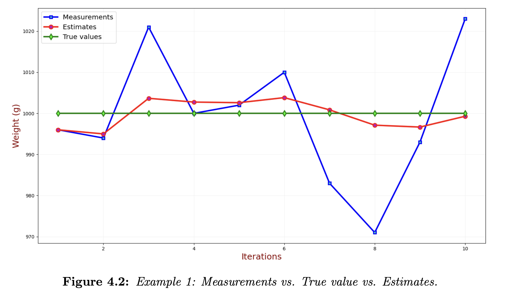
Recall the simple static state estimation example with weighing gold. We made multiple measurements and computed the estimate by averaging. We got the following results:

Estimate as a random variable

The difference between the estimates (red line) and the true values (green line) is the estimate error. The estimate error becomes lower as we make additional measurements, converging to zero, while the estimated value converges toward the true value. We don’t know the estimate error but we can estimate the state uncertainty.

The state estimate variance is denoted by $p$. This is also called the estimate uncertainty.

Measurement as a random variable

The measurement errors are the differences between the measurements (blue samples) and true values (green line). Since measurement errors are random, we can describe them by variance, ${\sigma }^2$. The standard deviation $\sigma$ of the measurement is the measurement uncertainty.

The measurement variance is denoted by $r$. This is also sometimes called the measurement error.

The variance of the measurement errors could be provided by the measurement equipment vendor, calculated, or derived empirically by a calibration procedure.

Let’s look at the weight measurements probability density function (PDF). The following plot shows 10 measurements of the gold bar weight.

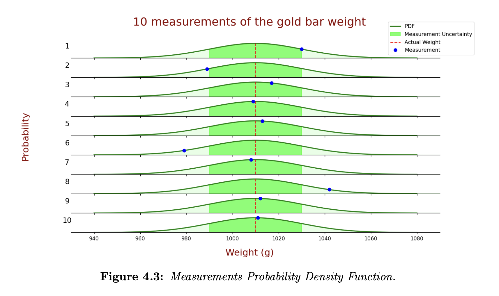
• The blue circles describe the measurements.
• The true values are at the red dashed line.
• The green line describes the probability density function of the measurement.
• The bold green area is the standard deviation $\sigma$ of the measurement – there is a probability of 68.26% that the measurement value lies within this area. 7 out of 10 the measurements are within the $1\sigma$ area.

State Prediction

In our simple static example of gold bar measurement, the weight of the gold bar is constant:

$${\hat{x}}_{n+1,n}={\hat{x}}_{n,n}$$

In the second example of constant velocity aircraft tracking, we extrapolated the current state (target position and velocity) to the next state using motion equations:

$$\begin{array}{rl}{\hat{x}}_{n+1,n}& ={\hat{x}}_{n,n}+\Delta t{\hat{\dot{x}}}_{n,n}\\ {\hat{x}}_{n+1,n}& ={\hat{\dot{x}}}_{n,n}\end{array}$$

Thus, we can see that the dynamic model equation depends on the system. Since the Kalman Filter treats the estimate as a random variable, we must extrapolate the estimate variance, $p_{n,n}$, to the next state as well.

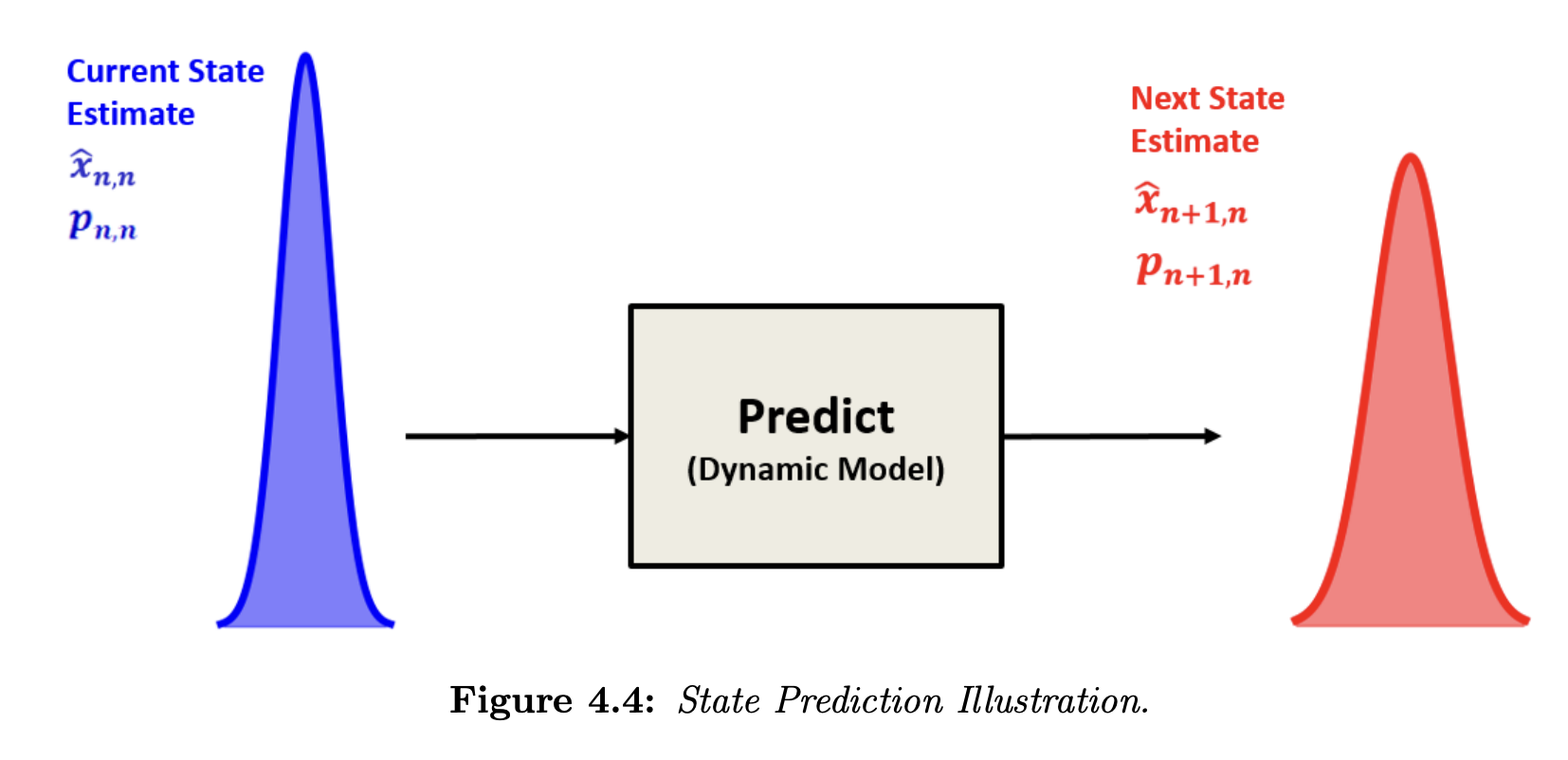
In the first static example, the dynamic model of the system is constant; thus, the estimate uncertainty extrapolation would be:

$${\hat{p}}_{n+1,n}=p_{n,n}$$

where $p$ is the estimate variance of the gold weight.

In the second constant velocity example, the estimate uncertainty extrapolation would be:

$$\begin{array}{rl}{p}_{n+1,n}^x& =p^x+\Delta t^2\cdot p_{n,n}^v\\ p_{n+1,n}^v& =p_{n,n}^v\end{array}$$

where $p^x$ is the position estimate variance and $p^v$ is the velocity estimate variance.

Why is it $\Delta t^2$? Note that for a normally distributed random variable $x$ with variance ${\sigma }^2$, $kx$ is normally distributed with variance $k^2{\sigma }^2$. Therefore, the time term in the uncertainty extrapolation equation is squared.

State Update

To estimate the current state of the system, we combine two random variables:

• The prior state estimate (current state estimate predicted at the previous state)
• The measurement

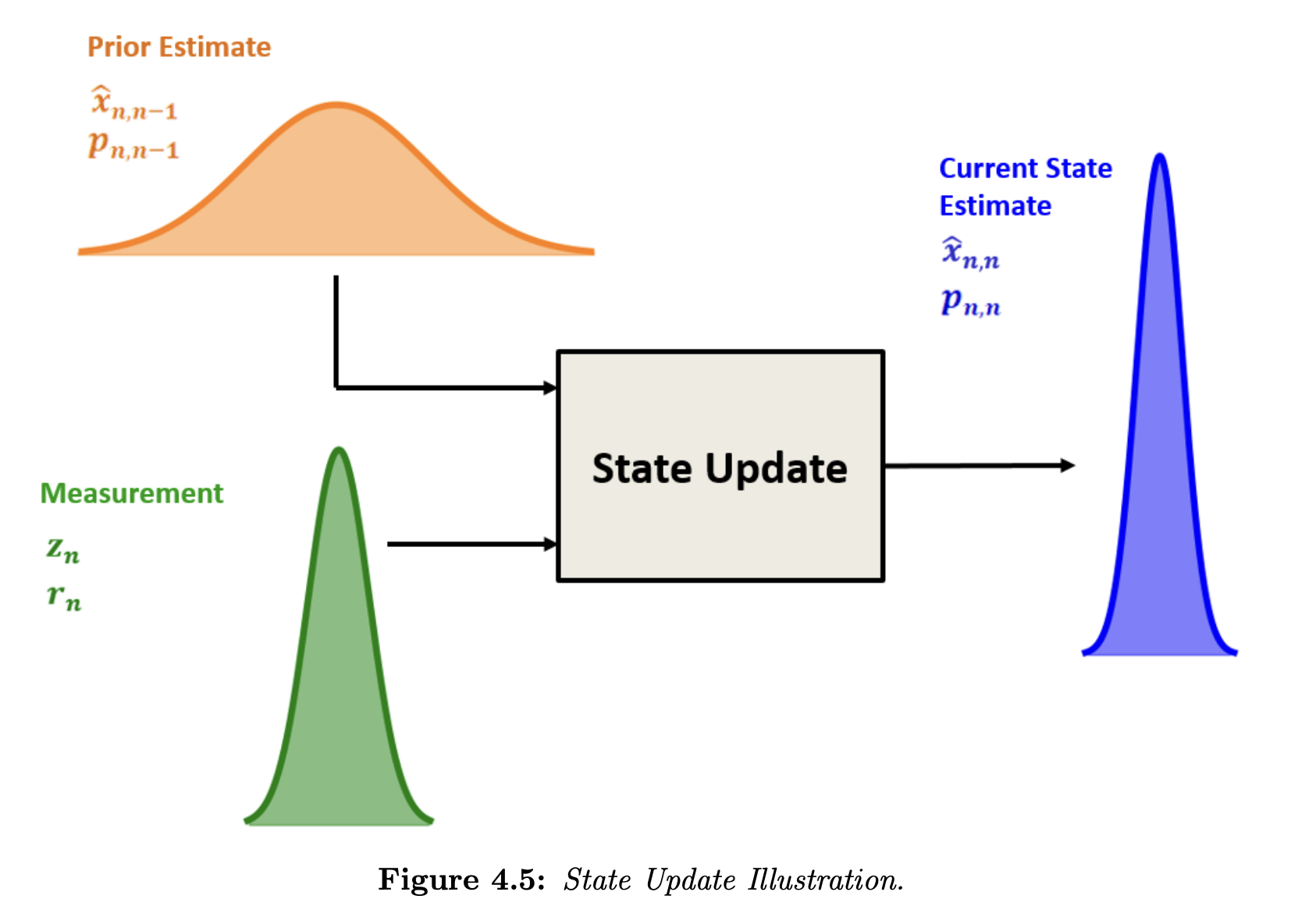
The Kalman filter is an optimal filter. It combines the prior state estimate with the measurement in a way that minimizes the uncertainty of the current state estimate.

The current state estimate is a weighted mean of the measurement and the prior state estimate:

$$\begin{array}{rl}& {\hat{x}}_{n,n}=w_1{z}_n+w_2{\hat{x}}_{n,n-1}\\ & w_1+w_2=1\end{array}$$

where $w_1,w_2$ are weights of the measurement $z_n$ and the prior state estimate ${\hat{x}}_{n,n-1}$. Alternatively, we can write it as:

$${\hat{x}}_{n,n}=w_1{z}_n+(1-w_1){\hat{x}}_{n,n-1}$$

The relationship between the variances is given as:

$$p_{n,n}=w_1^2{r}_n+(1-w_1{)}^2{p}_{n,n-1}$$

where:

• $p_{n,n}$ is the variance of the optimal combined estimate
• $p_{n,n-1}$ is the variance of the prior estimate ${\hat{x}}_{n,n-1}$
• $r_n$ is the variance of the measurement $z_n$

To find the $w_1$ that minimizes $p_{n,n}$, we differentiate $p_{n,n}$ with respect to $w_1$ and set the result to zero:

$$\frac{d{p}_{n,n}}{d{w}_1}=2w_1{r}_n-2(1-w_1)p_{n,n-1}=0$$

Solving:

$$\begin{array}{rl}{w}_1{r}_n& =p_{n,n-1}-w_1{p}_{n,n-1}\\ w_1{r}_n+w_1{p}_{n,n-1}& =p_{n,n-1}\\ w_1& =\frac{p_{n,n-1}}{r_n+p_{n,n-1}}\end{array}$$

Substituting into our current state estimation equation ${\hat{x}}_{n,n}$:

$$\begin{array}{rl}{\hat{x}}_{n,n}& =w_1{z}_n+(1-w_1){\hat{x}}_{n,n-1}\\ & =w_1{z}_n+{\hat{x}}_{n,n-1}-w_1{\hat{x}}_{n,n-1}\\ & ={\hat{x}}_{n,n-1}+w_1(z_n-{\hat{x}}_{n,n-1})\\ & =\frac{p_{n,n-1}}{r_n+p_{n,n-1}}(z_n-{\hat{x}}_{n,n-1})\end{array}$$

State Update Equation

$${\hat{x}}_{n,n}=\frac{p_{n,n-1}}{r_n+p_{n,n-1}}(z_n-{\hat{x}}_{n,n-1})$$

Recall that the innovation is $z_n-{\hat{x}}_{n,n-1}$. The weight of the innovation is the Kalman Gain:

$$\begin{array}{rl}{K}_n& =\frac{p_{n,n-1}}{r_n+p_{n,n-1}}\\ & =\frac{\text{Variance in estimate}}{\text{Variance in measurement}+\text{Variance in estimate}}\end{array}$$

The Kalman Gain is a number between $0$ and $1$:

$$0\le K_n\le 1$$

Finally, we need to find the variance of the current state estimate. We’ve seen that the relation between variances is given by:

$$p_{n,n}=K_n^2{r}_n+(1-K_n{)}^2{p}_{n,n-1}$$

where

$$1-K_n=1-\frac{p_{n,n-1}}{p_{n,n-1}+r_n}=\frac{p_{n,n-1}+r_n-p_{n,n-1}}{p_{n,n-1}+r_n}=\frac{r_n}{p_{n,n-1}+r_n}$$

Then, we can re-write the relation between variances as:

$$\begin{array}{rl}{p}_{n,n}& =K_n^2{r}_n+(1-K_n{)}^2{p}_{n,n-1}\\ & ={\left(\frac{p_{n,n-1}}{p_{n,n-1}+r_n}\right)}^2{r}_n+{\left(\frac{r_n}{p_{n,n-1}+r_n}\right)}^2{p}_{n,n-1}\\ & =\frac{p_{n,n-1}^2{r}_n}{(p_{n,n-1}+r_n{)}^2}+\frac{r_n^2{p}_{n,n-1}}{(p_{n,n-1}+r_n{)}^2}\\ & =\frac{p_{n,n-1}{r}_n}{p_{n,n-1}+r_n}\left(\frac{p_{n,n-1}}{p_{n,n-1}+r_n}+\frac{r_n}{p_{n,n-1}+r_n}\right)\\ & =(1-K_n)p_{n,n-1}(K_n+(1-K_n))\\ & =(1-K_n)p_{n,n-1}\end{array}$$

This is the Covariance Update Equation:

Covariance Update Equation

$$p_{n,n}=(1-K_n)p_{n,n-1}$$

It is clear from the equation that the estimate uncertainty is constantly decreasing with each filter iteration, since $(1-Kn)\le 1$.

• When the measurement uncertainty is high, the denominator of $K_n$ is large, resulting in a low Kalman Gain. Therefore, the convergence of the estimate uncertainty would be slow.
• On the other hand, the Kalman gain is high when the measurement uncertainty is low. Therefore, the estimate uncertainty would quickly converge toward zero.

Putting it all together

We combine the above pieces into a single algorithm.

The filter inputs are:

• Initialization: The initialization is only performed once. It provides two parameters:
  • Initial system state, ${\hat{x}}_{0,0}$
  • Initial state variance, $p_{0,0}$
• Measurement: The measurement is performed for every filter cycle, and it provides two parameters:
  • Measured system state, $z_n$
  • Measurement variance, $r_n$

The filter inputs are:

• System state estimate, ${\hat{x}}_{n,n}$
• Estimate variance, $p_{n,n}$

The following summarizes the five Kalman Filter equations.

State Update

$$\begin{array}{rl}{\hat{x}}_{n,n}& ={\hat{x}}_{n,n-1}+K_n(z_n-{\hat{x}}_{n,n})\\ p_{n,n}& =(1-K_n)p_{n,n-1}\\ K_n& =\frac{p_{n,n-1}}{p_{n,n-1}+r_n}\end{array}$$

State Predict

State

Constant system dynamics:

$$\begin{array}{r}{\hat{x}}_{n+1,n}={\hat{x}}_{n,n}\end{array}$$

Constant velocity:

$$\begin{array}{rl}{\hat{x}}_{n+1,n}& ={\hat{x}}_{n,n}+\Delta t{\hat{\dot{x}}}_{n,n}\\ {\hat{\dot{x}}}_{n+1,n}& ={\hat{\dot{x}}}_{n,n}\end{array}$$

Covariance

Constant system dynamics:

$$p_{n+1,n}^x=p_{n,n}^x$$

Constant velocity:

$$\begin{array}{rl}{p}_{n+1,n}^x& =p_{n,n}^x+\Delta t^2{p}_{n,n}^v\\ p_{n+1,n}^v& =p_{n,n}^v\end{array}$$

Note that the equations above don’t include the process noise. Process noise is added here.

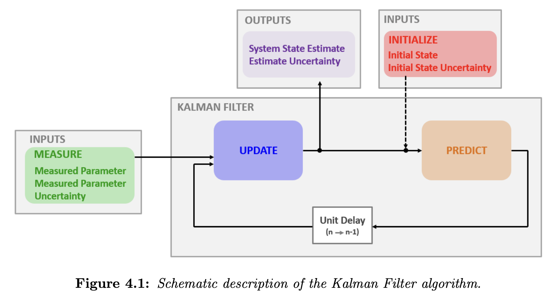
Block Diagram

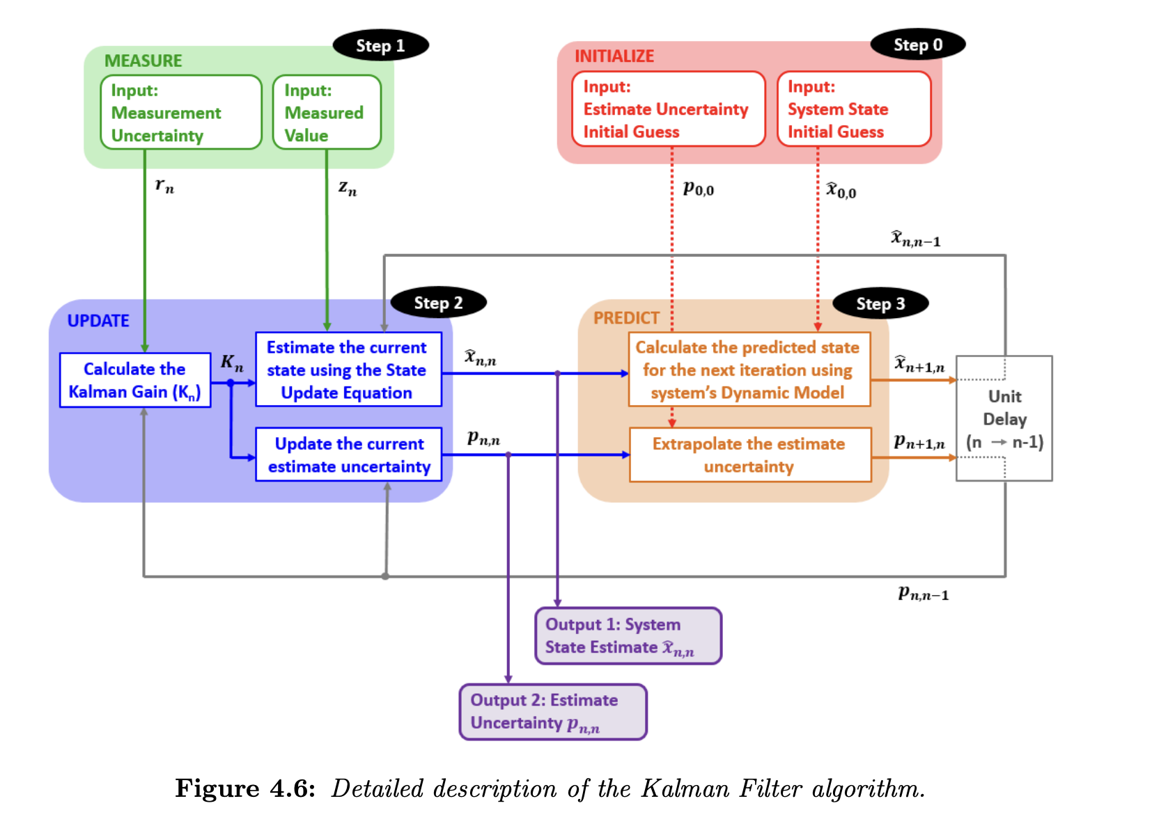
The general steps are described below.

Initialize. The initialization is performed only once, and it provides two parameters:

• Initial system state, ${\hat{x}}_{0,0}$
• Initial state variance, $p_{0,0}$

Measure. The measurement provides the following parameters:

• Measured system state, $z_n$
• Measured variance, $r_n$

State update. The state update process is responsible for the state estimation of the current state of the system:

• Measured value, $z_n$
• Measurement variance, $r_n$
• A prior predicted system state estimate, ${\hat{x}}_{n,n-1}$
• A prior predicted system state estimate variance, $p_{n,n-1}$

Based on the inputs, the state update process calculates the Kalman Gain and provides two outputs:

• Current system state estimate, ${\hat{x}}_{n,n}$
• Current state estimate variance, $p_{n,n}$

Predict. The prediction process extrapolates the current system state estimate and its variance to the next system state based on the dynamic model of the system. At the first filter iteration, the initialization is treated as the prior state estimate and variance. The prediction outputs are used as the prior (predicted) state estimate and variance on the following filter iterations.

Example: Estimating Building Height

In this example, we would like to estimate the height of a building using an imprecise altimeter.

We know that the building height doesn’t change over time (at least during the short measurement process).

Information given:

• The true height of the building is 50 meters.
• The altimeter measurement error (standard deviation) is 5 meters.
• The 10 measurements are: 49.03m, 48.44m, 55.21m, 49.98m, 50.6m, 52.61m, 45.87m, 42.64m, 48.26m, 55.84m.

Iteration 0

Initialization: The estimated height of the building based on the human eye we start from is:

$${\hat{x}}_{0,0}=60\text{ m}$$

A human estimation error is about $\sigma =15$. So, the variance is ${\sigma }^2=225\text{ m}$, so we have:

$$p_{0,0}=225$$

Prediction: Now, we predict the next state based on the initialization values. Since our system model is constant (the building doesn’t change height), we just have

$${\hat{x}}_{1,0}={\hat{x}}_{0,0}=60\text{ m}$$

The predicted variance also doesn’t change:

$$p_{1,0}=p_{0,0}=225$$

Iteration 1

Measurement: The first measurement is $49.03\text{ m}$. Since the standard deviation $\sigma$ of the altimeter measurement is 5, the variance ${\sigma }^2$ is $25$. Thus, the measurement uncertainty is $r_1=25$.

Update: We first calculate the Kalman Gain with:

$$K_1=\frac{p_{1,0}}{p_{1,0}+r_1}=\frac{225}{225+25}=0.9$$

Estimating the current state:

$$\begin{array}{rl}{\hat{x}}_{1,1}& ={\hat{x}}_{1,0}+K_1(z_1-{\hat{x}}_{1,0})\\ & =60+0.9(49.03-60)\\ & =50.13\text{ m}\end{array}$$

Updating the current estimate covariance:

$$\begin{array}{rl}{p}_{1,1}& =(1-K_1)p_{1,0}\\ & =(1-0.9)225\\ & =22.5\end{array}$$

Predict: Since the dynamic model of our system is constant, i.e., the building doesn’t change its height, we have

$${\hat{x}}_{2,1}={\hat{x}}_{1,1}=50.13\text{ m}$$

The extrapolated estimate variance also doesn’t change:

$$p_{2,1}=p_{1,1}=22.5$$

Iteration 2

After a unit time delay, the predicted estimate from the previous iteration becomes the prior estimate in the current iteration:

$${\hat{x}}_{2,1}=50.13\text{ m}$$

The extrapolated estimate becomes the prior estimate variance:

$$p_{2,1}=22.5$$

Measure: The second measurement is $z_2=48.44\text{ m}$. The measurement variance is $r_2=25$.

Update: The Kalman Gain calculation is

$$K_2=\frac{p_{2,1}}{p_{2,1}+r_2}=\frac{22.5}{22.5+25}=0.47$$

Estimating the current state:

$$\begin{array}{rl}{\hat{x}}_{2,2}& ={\hat{x}}_{2,1}+K_2(z_2-{\hat{x}}_{2,1})\\ & =50.13+0.47(48.44-50.13)\\ & =49.33\text{ m}\end{array}$$

Updating the current estimate variance:

$$\begin{array}{rl}{p}_{2,2}& =(1-K_1)p_{2,1}\\ & =(1-0.47)22.5\\ & =11.84\end{array}$$

Predict: Since the dynamic model of our system is constant, i.e., the building doesn’t change its height, we have

$${\hat{x}}_{3,2}={\hat{x}}_{2,2}=49.33\text{ m}$$

The extrapolated estimate variance also doesn’t change:

$$p_{3,2}=p_{2,2}=11.84$$

Results & Analysis

First of all, we want to ensure Kalman Filter convergence. The Kalman Gain should gradually decrease until it reaches a steady state. When Kalman Gain is low, the weight of the noisy measurements is also low. The following plot describes the Kalman Gain for the first one hundred iterations of the Kalman Filter.

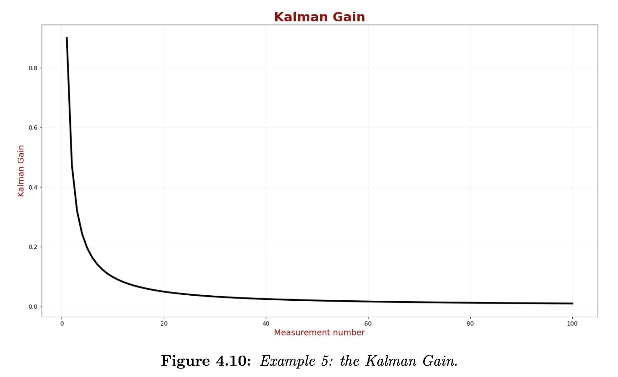
We can see a significant reduction in the Kalman Gain in the first 10 iterations; a steady state is hit after about 50 iterations.

The estimation error is the difference between the true values (the green line) and the KF estimates (the red line). We can see that the estimation errors of our KF decrease in the filter convergence region.

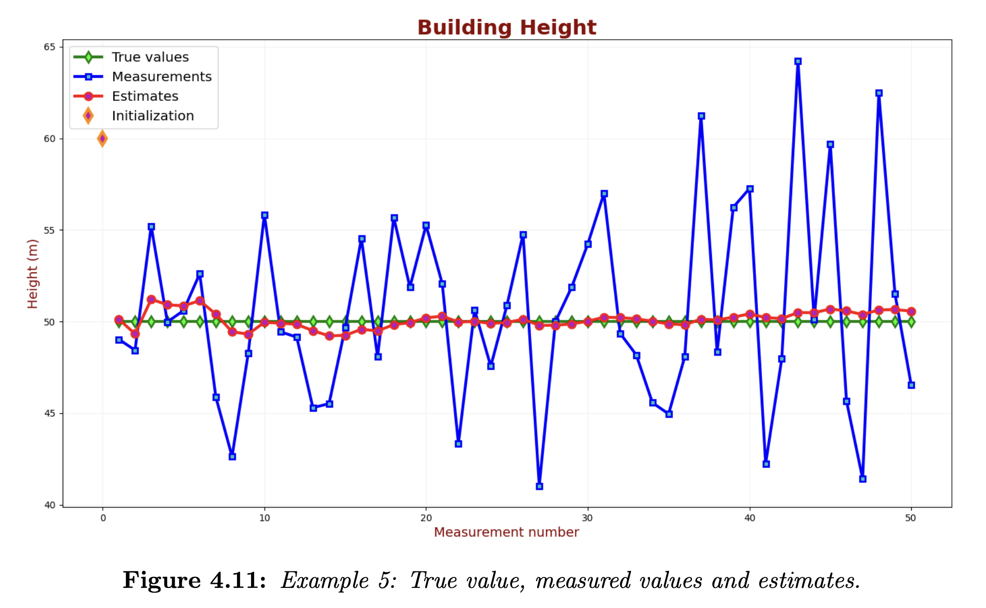
The typical accuracy criteria are maximum error, mean error, and root mean square error.

Another important parameter is estimation uncertainty. We want the Kalman Filter (KF) estimates to be precise; therefore, we are interested in low estimation uncertainty.

Assume that for a building height measurement application, there is a requirement for 95% confidence. The following chart shows the KF estimates and the true values with 95% confidence intervals.

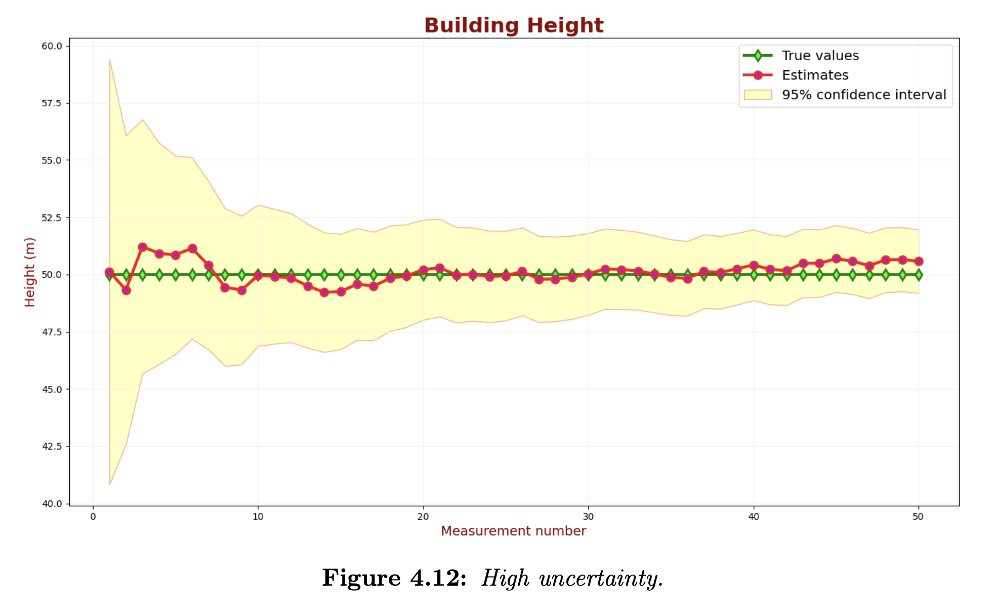
In the above chart, the confidence intervals are added to the estimates (the red line). 95% of the green samples should be within the 95% confidence region.

We can see that the uncertainty is too high. Let us decrease the measurement uncertainty. The following chart describes the KF output for a low measurement uncertainty parameter.

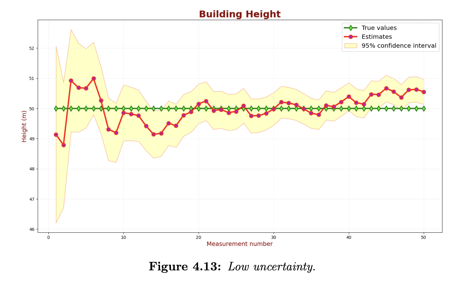
Although we’ve decreased the uncertainty of the estimates, many green samples are outside the 95% confidence region. The Kalman Filter is overconfident and too optimistic about its accuracy.

Let us find the measurement uncertainty that yields the desired estimate uncertainty.

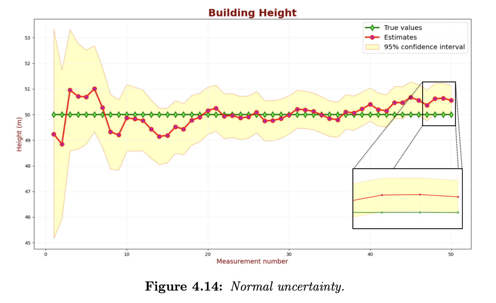
The above chart shows that 2 out of 50 samples slightly exceed the 95% confidence region. This performance satisfies our requirements.