Linearization of Nonlinear State Space Models

How do we linearize about $(x_e,\overline{u})$, which is an equilibrium point?

$$\begin{array}{r}\dot{x}=f(x,u)\\ y=g(x,u)\end{array}$$

We can approximate the nonlinear functions using a first-order Taylor expansion:

$$\begin{array}{r}f(x,u)\approx f(x^e,\overline{u})+\frac{\partial f}{\partial x}{|}_{(x_e,\overline{u})}(x-x^e)+\frac{\partial f}{\partial u}{|}_{(x_e,\overline{u})}(u-\overline{u})\\ g(x,u)\approx g(x^e,\overline{u})+\frac{\partial g}{\partial x}{|}_{(x_e,\overline{u})}(x-x^e)+\frac{\partial g}{\partial u}{|}_{(x_e,\overline{u})}(u-\overline{u})\end{array}$$

Then, we can write it as a vector

$$f(x,u)=\left[\begin{array}{c}{f}_1(x,u)\\ ⋮\\ f_n(x,u)\end{array}\right],x=\left[\begin{array}{c}{x}_1\\ ⋮\\ x_n\end{array}\right]$$

Then, we can write the Jacobians, which are the local slopes of the nonlinear system.

$$\begin{array}{r}\frac{\partial f}{\partial x}:=\left[\begin{array}{ccc}\frac{\partial f_1}{\partial x_1}& \dots & \frac{\partial f_1}{\partial x_n}\\ ⋮& \ddots & ⋮\\ \frac{\partial f_n}{\partial x_1}& \dots & \frac{\partial f_n}{\partial x_n}\end{array}\right],\frac{\partial f}{\partial u}:=\left[\begin{array}{c}\frac{\partial f_1}{\partial u}\\ ⋮\\ \frac{\partial f_n}{\partial u}\end{array}\right]\\ \frac{\partial g}{\partial x}:=\left[\begin{array}{ccc}\frac{\partial g}{\partial x_1}& \dots & \frac{\partial g}{\partial x_n}\end{array}\right],\frac{\partial g}{\partial u}:=\frac{\partial g}{\partial u}\end{array}$$

Re-visiting the pendulum from Nonlinear State Space Models, where we have $n=\dim x=2$:

$$\begin{array}{rl}f& =\left[\begin{array}{c}{f}_1\\ f_2\end{array}\right]=\left[\begin{array}{c}{x}_2\\ -\frac{g}{l}\sin x_1-\frac{D}{ml}{x}_2+\frac{1}{ml}u\end{array}\right]\\ g& =x_1\\ \frac{\partial f}{\partial x}& =\left[\begin{array}{cc}\frac{\partial f_1}{\partial x_1}& \frac{\partial f_1}{\partial x_2}\\ \frac{\partial f_2}{\partial x_1}& \frac{\partial f_2}{\partial x_2}\end{array}\right]=\left[\begin{array}{cc}0& 1\\ -\frac{g}{l}\cos x_1& -\frac{D}{ml}\end{array}\right]\\ \frac{\partial f}{\partial u}& =\left[\begin{array}{c}\frac{\partial f_1}{\partial u}\\ \frac{\partial f_2}{\partial u}\end{array}\right]=\left[\begin{array}{c}0\\ \frac{1}{ml}\end{array}\right]\\ \frac{\partial g}{\partial x}& =\left[\begin{array}{cc}\frac{\partial g}{\partial x_1}& \frac{\partial g}{\partial x_2}\end{array}\right]=\left[\begin{array}{cc}1& 0\end{array}\right]\\ \frac{\partial g}{\partial u}& =0\end{array}$$

This will then give us

$$\dot{x}=\cancel{f(x^e,\overline{u})}+\underset{A}{\underbrace{\left[\begin{array}{cc}0& 1\\ -\frac{g}{l}{x}_1^e& -\frac{D}{ml}\end{array}\right]}}\underset{\Delta x}{\underbrace{\left[\begin{array}{c}{x}_1-x_1^e\\ x_2-x_2^e\end{array}\right]}}+\underset{B}{\underbrace{\left[\begin{array}{c}0\\ \frac{1}{ml}\end{array}\right]}}\underset{\Delta u}{\underbrace{(u-\overline{u})}}$$

• The first term is 0 because of the definition of an equilibrium point

So, if we define the deviation from the equilibrium point as $\Delta x=x-x^e$, we can write

$$\dot{\Delta x}=\dot{(x-x^e)}=\dot{x}=A\Delta x+B\Delta u$$

Similarly, for $y$:

$$y=g(x,u)\approx g(x_e,\overline{u})+\underset{C}{\underbrace{\left[\begin{array}{cc}1& 0\end{array}\right]}}\underset{\Delta x}{\underbrace{\left[\begin{array}{c}{x}_1-x_1^e\\ x_2-x_2^e\end{array}\right]}}+\underset{D}{\underbrace{0}}\underset{\Delta u}{\underbrace{(u-\overline{u})}}$$

such that

$$\Delta y:=y-g(x^e,\overline{u})=C\Delta x+D\Delta u$$

Thus, for the entire system:

$$\begin{array}{rl}\dot{\Delta x}& =A\Delta x+B\Delta u\\ \Delta y& =C\Delta x+D\Delta u\end{array}$$

Thus, we can see that linearization about an equilibrium point leads to an LTI system.

For our pendulum case, consider fixing $\overline{u}=0$. This results in two equilibria:

$$x^{e,s}=\left[\begin{array}{c}0,0\end{array}\right],x^{e,u}=\left[\begin{array}{c}0\\ \pi \end{array}\right]$$

Consider the linearization about $x^{e,u}$:

$$\begin{array}{rl}\dot{\Delta x}& =\underset{A}{\underbrace{\left[\begin{array}{cc}0& 1\\ \frac{g}{l}& -\frac{D}{ml}\end{array}\right]}}\Delta x+\underset{B}{\underbrace{\left[\begin{array}{c}0\\ \frac{1}{ml}\end{array}\right]}}\Delta u\\ \Delta y& =\underset{C}{\underbrace{\left[\begin{array}{cc}1& 0\end{array}\right]}}\Delta x\end{array}$$

Assume $\Delta u=0\forall t\ge 0$. Then, we would have

$$\dot{\Delta x}=\left[\begin{array}{cc}0& 1\\ \frac{g}{l}& -\frac{D}{ml}\end{array}\right]\Delta x$$

where $A$ has one stable eigenvalue ${\lambda }^s$ with eigenvector $v^s$ and 1 unstable eigenvalue ${\lambda }^u$ with eigenvector $v^u$. The state space is shown below.

• Blue line is $\text{span}(v^s)$ and red line is $\text{span}(v^u)$.

Definition: Stable equilibrium point

An equilibrium point $x^e$ is stable if all of the eigenvalues of the linearization at $x^e$ ($A=\frac{\partial f}{\partial x}{|}_{(x^e,\overline{u})}$) are stable (in ${\mathbb{C}}^{-}$).

Note that $x^{e,u}$ is an unstable equilibrium point because it has an unstable eigenvalue ${\lambda }^u$.

Consider the linearization about $x^{e,s}$:

$$\begin{array}{rl}\dot{\Delta x}& =\underset{A}{\underbrace{\left[\begin{array}{cc}0& 1\\ -\frac{g}{l}& -\frac{D}{ml}\end{array}\right]}}\Delta x+\underset{B}{\underbrace{\left[\begin{array}{c}0\\ \frac{1}{ml}\end{array}\right]}}\Delta u\\ \Delta y& =\underset{C}{\underbrace{\left[\begin{array}{cc}1& 0\end{array}\right]}}\Delta x\end{array}$$

• The difference is $\frac{g}{l}$ is negative here.

Assume $\Delta u=0\forall t\ge 0$. Then, we would once again have:

$$\dot{\Delta x}=A\Delta x$$

where $A$ has 2 stable eigenvalues:

• Eigenvalue ${\lambda }^s=\text{Re}({\lambda }^s)+j\text{Im}({\lambda }^s)$ with eigenvector $v^s$
• Eigenvalue $\overline{{\lambda }^s}$ with eigenvector $\overline{v^s}$

Thus, $x^{e,s}$ is a stable equilibrium point. The state space is shown below.

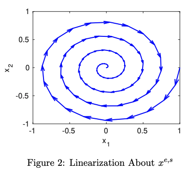
If we have $\overline{u}\in (0,mg)$, we will have 2 equilibria. The nonlinear state space is shown below:

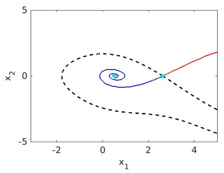
$x^{e,s}$ represents a desired operating point. The region inside the dashed line is the region of attraction of $x^{e,s}$, which represents a safe operating region.

Definition: Region of Attraction

The region of attraction of $x^{e,s}$ is the set of initial conditions $x_0$ such that $x(t=0)=x_0$ implies that ${\lim }_{t\to \infty }x(t)=x^{e,s}$.

The unstable trajectory from the above state space looks like this: