Shattered Gradients

Sequential processing

Basic neural networks do sequential data processing, where the output of each layer is passed directly to the next layer. For example, a 3-layer sequential network would be defined as:

$$\begin{array}{rl}{h}_1& =f_1[x,{\varphi }_1]\\ h_2& =f_2[h_1,{\varphi }_2]\\ h_3& =f_3[h_2,{\varphi }_3]\\ y& =f_4[h_3,{\varphi }_4]\end{array}$$

where $h_1,h_2,h_3$ are computed intermediate hidden layers, $x$ is the input, $y$ is the output, and $f_k[\bullet ,{\varphi }_k]$ is the processing function.

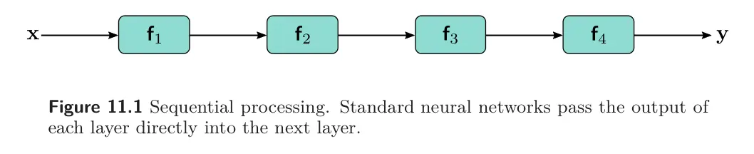
In a standard fully-connected neural network, $f_k$ computes a linear transformation followed by an activation function, and the parameters ${\varphi }_k$ consist of weights and biases of the linear transformation. In a convolutional neural network, $f_k$ applies the convolution operation, and ${\varphi }_k$ consist of convolution kernel weights and biases.

We can alternatively think of this network as a nested function:

$$y=f_4\left[f_3\right[f_2[f_1[x,{\varphi }_1],{\varphi }_2],{\varphi }_3],{\varphi }_4]$$

Limitations of sequential processing

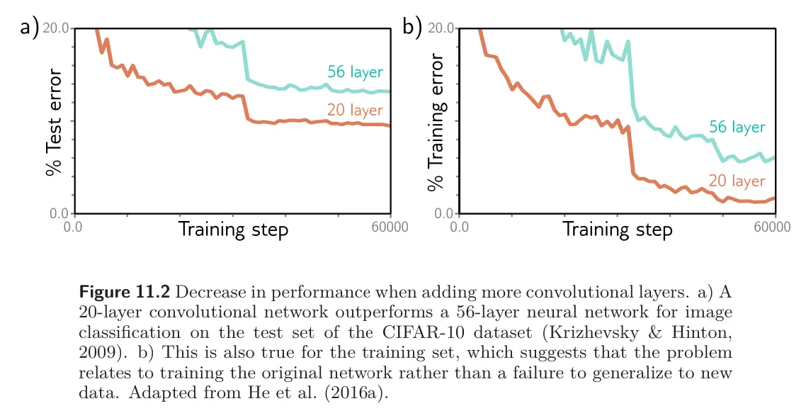
In principle, we can add as many layers as we want; we’ve seen that adding more layers does improve performance, as in the case of VGG vs. AlexNet. However, image classification performance decreases again as further layers are added (see Figure 11.2). This is surprising considering that double descent tells us that over-parameterized models still perform better. The decrease in performance is present for both the training set and testing set, which implies that the problem is training deeper networks, rather than inability to generalize.

This phenomenon is not complete understood. One conjecture is that at initialization, the loss gradients change unpredictably when we modify parameters in early network layers. With appropriate weight initialization, the gradient of the loss with respect to these parameters will be reasonable (no exploding gradient). However, the derivative assumes an infinitesimal change in the parameter, whereas our optimization uses a finite step-size. Any reasonable choice of step size may move to a place with a completely different and unrelated gradient; the loss surface looks like a range of tiny mountains rather than a smooth structure. Thus, we don’t make progress in the way that we do when the loss function gradient changes more slowly.

This conjecture is supported by empirical observations of gradients in networks with a single input and output. For a shallow network, the gradient of the output with respect to the input changes slowly as we change the input. However, for a deep network, a tiny change in the input results in a completely different gradient. This is captured by the autocorrelation function of the gradient; nearby gradients are correlated for shallow networks, but this correlation quickly drops to zero for deep networks. This is termed the shattered gradients phenomenon.

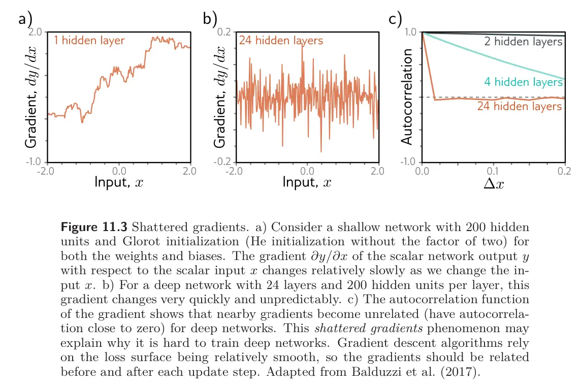
Autocorrelation function

The autocorrelation $r[\tau ]$ of a continuous function $f[z]$ is defined as:

$$r[\tau ]={\int }_{-\infty }^{\infty }f[t+\tau ]f[t]dt$$

where $\tau$ is the time lag. Sometimes, this is normalized by $r[0]$ so that the autocorrelation at time lag zero is one.

The autocorrelation function is a measure of the correlation of the function with itself as a function of an offset (i.e., the time lag). If a function changes slowly and predictably, then the autocorrelation function will decrease slowly as the time lag increases from zero. If the function changes fast and unpredictably, then it will decrease quickly to zero.

Shattered gradients presumably arise because changes in early network layers modify the output in an increasingly complex way as the network becomes deeper. The derivate of the output with respect to the first layer $f_1$ for our sequential network is:

$$\frac{\partial y}{\partial f_1}=\frac{\partial f_2}{\partial f_1}\frac{\partial f_3}{\partial f_2}\frac{\partial f_4}{\partial f_3}$$

When we change the parameters that determine $f_1$, all of the derivatives in this sequence are evaluated at slightly different locations since layers $f_2,f_3,f_4$ are themselves computed from $f_1$. Consequently, the updated gradient at each training example may be completely different, and the loss function becomes badly behaved.