We have seen that bias-variance tradeoff occurs as we increase the capacity of a model. However, in practice, the phenomenon of double descent can occur.
Example
Consider a case where we train on the MNIST-1D dataset with 10,000 training examples and 5,000 testing examples. We train the model with Adam and a step size of 0.005 using a full batch of 10,000 examples for 4000 steps, and examine the train/test performance as we increase the capacity (number of parameters) of the model.
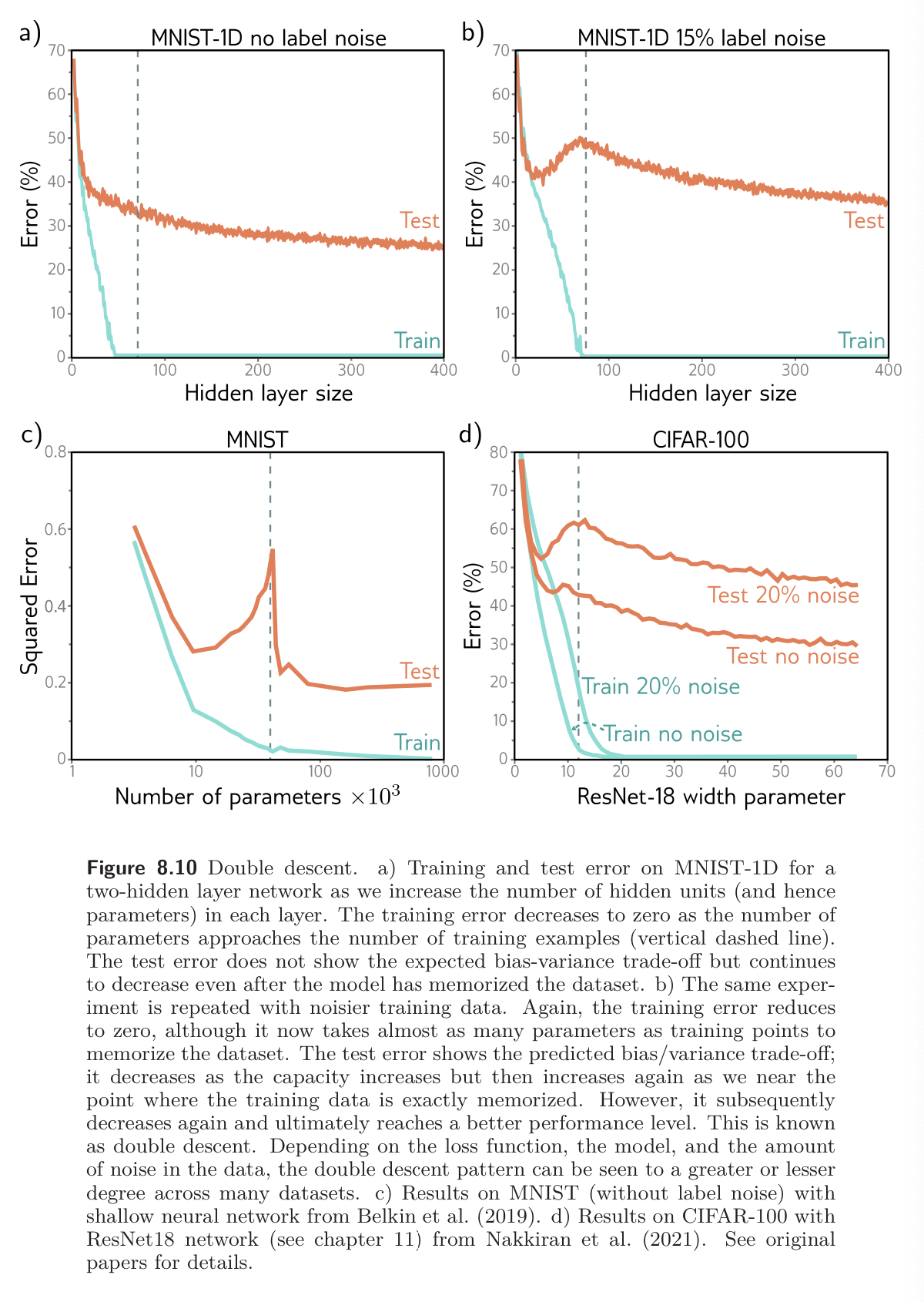
Part (a) of the figure shows the training and test error for a neural network with two hidden layers as the number of hidden units increases. The training error decreases as the capacity grows and quickly becomes closer to zero. The vertical dashed represents the capacity where the model has the same number of parameters as there are training examples, but the model memorizes the dataset before this point. The test error decreases as we add model capacity but does not increase as predicted by the bias-variance tradeoff; it keeps decreasing.
Part (b) repeats the experiment but this time we randomize 15% of the training labels. Training error decreases to zero again. Due to more randomness, the model requires almost more parameters (almost as many as data points) to memorize the data. The test error does show the bias-variance tradeoff as we increase the capacity to the point where the model fits the training data exactly. However, it then unexpectedly begins to decrease again. If we add enough capacity, the test loss reduces to below the minimal level that we achieved in the first part of the curve.
This is called double descent. For some datasets like MNIST (fig 8.10c), it’s present with the original data. For others, like MNIST-1D and CIFAR (fig 8.10d), it emerges when we add noise to labels.
Parts of the curve:
- First part: Classical or under-parametrized regime
- Central part (where error increases): Critical regime
- Second part: Modern or over-parametrized regime
Explanation
Double descent is recent, unexpected, and somewhat puzzling. It results from an interaction of two phenomena:
- The test performance becomes temporarily worse when the model has just enough capacity to memorize the data. This is exactly as predicted by the bias-variance tradeoff.
- The test performance continues to improve with capacity even when this exceeds the point where all the training data are classified correctly. This phenomenon is confusing; it’s unclear why performance should be better in the over-parametrized regime, given there are not even enough training data points to constrain the model parameters uniquely.
To understand why performance continues to improve as we add more parameters, note that once the model has enough capacity to drive the training loss to near zero, the model fits the training data almost perfectly. This implies that further capacity cannot help the model fit the training data any better; any change must occur between training points. The tendency of a model to prioritize one solution over another as it extrapolates between data points is known as inductive bias.
The model’s behavior behavior between data points is critical because training data is extremely sparse in high-dimensional space. MNIST-1D data is 40-dimensional, and we trained with 10,000 examples. Consider what would happen if we quantized each input dimension into 10 bins. There would be bins in total, constrained by only examples. Even with this coarse quantization, there will only be one data point in every bins. This tendency of the volume of high-dimensional space to overwhelm the number of training points is called the Curse of Dimensionality.
The implication is that problems in high dimensions might look like figure 8.11a below; there are small regions of the input space where we observe data, with significant gaps between them.
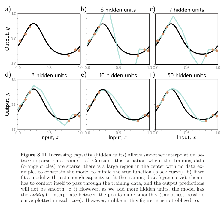
Thus, the putative explanation for double descent is that as we add capacity to the model, it interpolates between the nearest data points increasingly smoothly. In the absence of information about what happens between the training points, assuming smoothness is sensible and will probably generalize reasonably to new data.
This argument is plausible. It’s true that as we add more capacity to the model, it will have the capability to create smoother functions. Figure 8.11b-f show the smoothest possible functions that still pass through the data points as we increase the number of hidden units. In Figure 8.11b, when the number of parameter is close to the number of training data examples (not yet overparametrized), the model is forced to contort itself to fit the training data exactly, resulting in erratic predictions. This explains why the peak in the double descent curve is so pronounced. As we add more hidden units, the model has the ability to construct smoother functions that are likely to generalize better to new data.
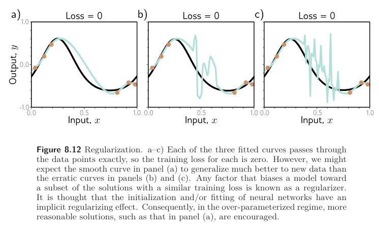
However, this does not explain why overparametrized models should produce smooth functions. Figure 8.12 shows three functions that can be created by the simplified model with 50 hidden units. In each case, the model fits the data exactly, so the loss is zero. If the modern regime of double descent is explained by increasing smoothness, then what exactly encouraging this smoothness? The answer to this is uncertain, but there are two likely possibilities:
- The network initialization may encourage smoothness, and the model never departs from the sub-domain of smooth function during the training process.
- The training algorithm may somehow “prefer” to converge to smooth functions. Any factor that biases a solution toward a subset of equivalent solutions is known as a regularizer, so one possibility is that the training algorithm acts as an implicit regularizer (see Implicit Regularization).
Further Notes
It has been empirically shown that test performance depends on the effective model capacity (the largest number of samples for which a given model and training method can achieve zero training error). At this point, the model starts to devote its efforts to interpolating smoothly. As such, the test performance depends not just on the model but also on the training algorithm and length of training. The same pattern has been observed when studying a model with fixed capacity and increasing the number of training iterations. This is called epoch-wise double descent.
Double descent makes the strange prediction that adding training data can sometimes worse test performance. Consider an over-parameterized model in the second descending part of the curve. If we increase the training data to match the model capacity, we will now be in the critical region of the new test error curve, and the test loss may increase.
It’s been shown (see here) that overparameterization is necessary to interpolate data smoothly in high dimensions. They demonstrate a tradeoff between the number of parameters and the Lipschitz constant of the model (the fastest the output can change for a small input change).