Using gradient descent to find the global optimum of a high-dimensional loss function is challenging, especially in non-convex cases. We can find a minimum, but there is no way to tell if this is a global minimum or even a good one.
One of the main problems is that the final destination of vanilla gradient descent is entirely determined by the starting point. Stochastic gradient descent attempts to remedy this by adding some noise to the gradient at each step. The solution still moves downhill on average, but at any given iteration, the direction chosen is not necessarily in the steepest downhill direction - it may not be downhill at all. Thus, SGD can possibly move uphill temporarily and hence jump from one “valley” of the loss function to another.
The mechanism for introducing randomness is to use a random subset (batch) and compute the gradient from these, instead of using the whole dataset.
Batches & Epochs
At each iteration, the algorithm chooses a random subset (“minibatch” or “batch”) of the training data and computes the gradient from these examples alone. The update rule for model parameters at time is hence:
where:
- is a set containing the indices of the input/output pairs in the current batch
- is the loss due to the -th pair of {training sample, ground truth}.
- is the learning rate; together with the gradient magnitude, it determines the distance moved at each iteration. This is chosen at the start of the algorithm and does not depend on the local properties of the function.
Batches are usually drawn from the dataset without replacement. The algorithm works through the training examples until it has used all the data, at which point it starts sampling from the full training dataset again. A single pass through the entire training dataset is referred to as an epoch.
- A batch may be as small as a single example or as large as the entire dataset. The latter is called full-batch gradient descent and is identical to vanilla (non-stochastic) gradient descent.
Variable Loss Function View
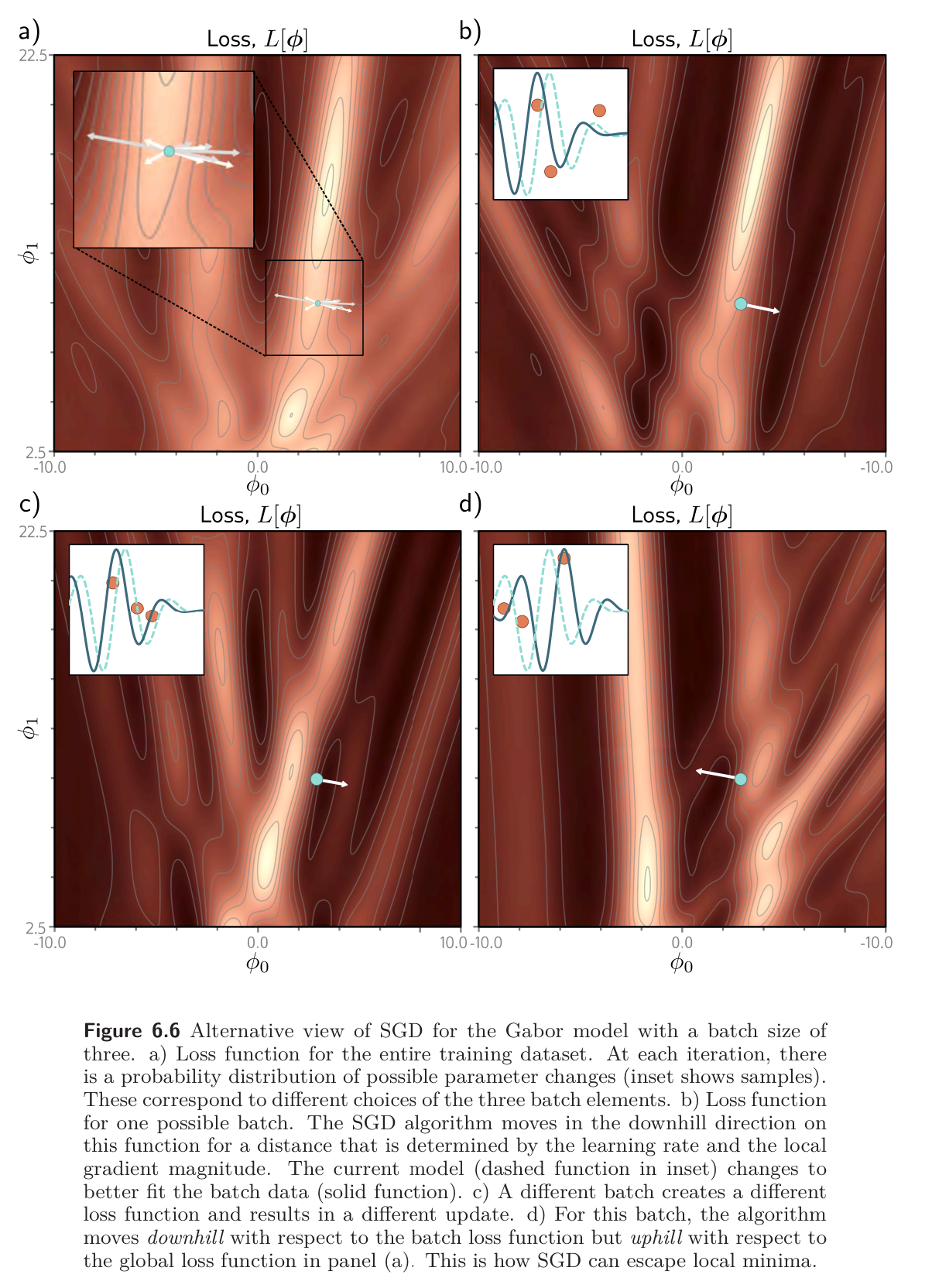
An alternative interpretation of SGD is that it computes the gradient of a different loss function at each iteration; the loss function depends on both the model and the training data and hence will differ for each randomly selected batch. In this view, SGD performs deterministic gradient descent on a constantly changing loss function. Despite this variability, the expected loss and expected gradients at any point remain the same as for gradient descent.
This view shows us how SGD lets us escape local minima – while we may have reached a local minima for one loss function, the next batch has a “new” loss function which might shoot us in a different direction.
Properties of SGD
SGD has several attractive features:
- Although it adds noise to the trajectory, it still improves the fit to a subset of the data at each iteration. Hence, the updates tend to be sensible even if they are not optimal.
- Because it draws training examples without replacement and iterates through the dataset, the training examples all still contribute equally.
- It is less computationally expensive to compute the gradient for just a subset of the training data.
- It can escape local minima in principle.
- Taking samples from the gradient at some point might bounce you around the landscape and out of the local optima.
- It reduces the chances of getting stuck near saddle points; it’s likely that at least some of the possible batches will have a significant gradient at any point on the loss function.
- There is some evidence that SGD finds parameters for neural networks that cause them to generalize well to new data in practice.
- Sometimes, optimizing the network to the training data really well is not what we want to do, because it might overfit the training set; so, in fact, SGD might not get lower training error than GD, it might result in lower test error.
- Taking a bunch of small steps in a stochastic manner tends to average out to about the same as naive gradient descent.
Convergence
SGD does not necessarily converge in a traditional sense. The hope is that when we are close to the global medium, all data points will be well described by the model. As such, the gradient will be small for whatever batch is chosen, and the parameters will not change much.
In practice, SGD is often applied with a learning rate schedule – The learning rate starts at a high value and is decreased by a constant factor every epochs. - In the early stages of training, we want the algorithm to explore the parameter space, jumping from valley to valley to find a sensible region. In later stages, we are roughly in the right place and are more concerned with fine-tuning the parameters, so we decrease to make smaller changes.
Theorem: Step size and convergence
If is convex and is a sequence satisfying
then SGD converges with probability to the optimal .
An example of decreasing step size would be to make but people often use rules that decrease slowly, and so don’t strictly satisfy the criteria for convergence.