The root locus method is a graphical method for examining how the roots of a system change with variation of a certain system parameter.
Set-up
Consider the unity feedback configuration:
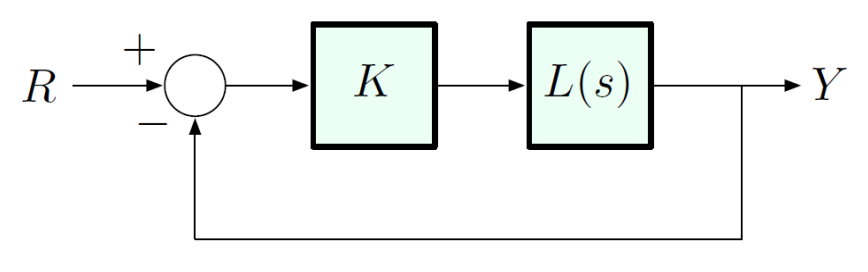
where is a constant gain and where and are some polynomials.
The closed-loop transfer function is:
so the closed-loop poles are the solutions of
This is called the characteristic polynomial and setting it to zero gives us the characteristic equation.
Note: Change of Notation
Here we have changed from or to . This is because the root-locus method is quite general, so is not necessarily the plant transfer function, and is not necessarily the feedback gain. These two may be related to the plant transfer function and feedback through some transformation. As long as we can represent the poles of the closed-loop transfer function as roots of the equation for some choice of and , we can apply the root-locus method.
The Routh Criterion gave us a range of to guarantee stability. However, for what values of do we best satisfy given design specs, like setting time, rise time, and overshoot? These specs are encoded in pole locations.
Root locus
The root locus for is the set of all closed-loop poles, i.e., the roots of as varies from to .
An equivalent characterization of the root locus concept is to use the “phase condition”. The root locus for the characteristic equation is the set of all values of that make this equation true as varies from to . Another way to think about this is:
Since , this implies that must be a negative real number. Thus, a point lies on the root locus if and only if . In other words, must be real and negative. This is called the phase condition.
See a simple example of root locus method here, where we analytically draw a root locus plot for a 2nd-order system. However, for order larger than 2, there will generally be no direct formula for the closed-loop poles as a function of . Thus, we develop simple rules for (approximately) sketching the root locus in the general case.
Rule A – Number of Branches
The characteristic equation can be written as:
Since , the characteristic polynomial has degree .
The characteristic polynomial has solutions (roots), some of which repeated. As we vary , these solutions also vary to form branches.
More succinctly:
Rule A
Rule B – Start Points
The locus starts from . What happens near ? We see that if and , then . Therefore:
- is close to a root of , or
- is close to a pole of .
Rule B
Rule C – End Points
What happens to the locus at ?
Thus, as ,
- Branches end at the roots of , or
- Branches end at zeros of
Rule C
Note: If , we have branches but only zeros. The remaining branches go off to infinity (end at “zeros at infinity”).
Rule D – Real Locus
The branches of the root locus start at the open-loop poles. Which way do they go, left or right?
Recall that phase condition:
Thus,
This sum must be for any that lies on the root locus.
See this example to see how this works in practice.
Rule D
If is real, then it is on the real line of if and only if there are an odd number of real open-loop poles and zeros to the right of .
Rule E – Asymptotes
How does the locus as ?
Claim: If , then
Proof of the above claim:
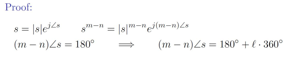
Rule E
Thus, Rule E tells us that branches near have phase
Note that if , then there are no branches at .
Rule F: Imaginary Axis Crossing
Do the branches of the root locus cross the axis? This signifies a transition from stability to instability.
Our goal is to determine if the equation
has a solution for some .
Rule F
Use Routh Criterion to first determine the critical value of (when the characteristic polynomial becomes unstable), then plug it in and solve for -crossing (numerically or analytically).