Simple Root Locus Example

Consider a system where we have

$$L(s)=\frac{1}{s^2+s}$$

such that $L(s)=\frac{b(s)}{a(s)}$ where $b(s)=1$ and $a(s)=s^2+s$.

The characteristic equation is $a(s)+Kb(s)=0$, giving us

$$s^2+s+K=0$$

Using the quadratic formula to solve the characteristic equation gives us

$$s=-\frac{1\pm \sqrt{1-4K}}{2}=-\frac{1}{2}\pm \frac{\sqrt{1-4K}}{2}$$

Thus, the root locus are

$$\text{Root locus}=\left\{-\frac{1}{2}\pm \frac{\sqrt{1-4K}}{2}:0\le K<\infty \right\}\subset \mathbb{C}$$

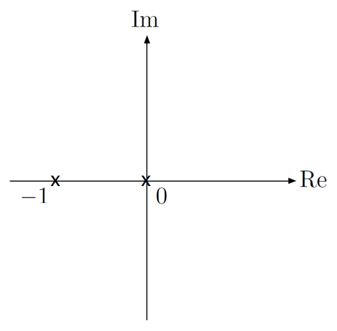
Let’s plot this in the $s$-plane. We start from $K=0$, where the roots are $-\frac{1}{2}\pm \frac{1}{2}=-1,0$.

• Note that these are poles of $L$ (open-loop poles).

As $K$ increases from $0$, the poles start to move:

$$\begin{array}{rl}1-4K>0& ⟹\text{2 real roots}\\ K=\frac{1}{4}& ⟹\text{1 real root at }s=-\frac{1}{2}\end{array}$$

For $K>\frac{1}{4}$, we have 2 complex roots with $\text{Re}(s)=-\frac{1}{2}$.

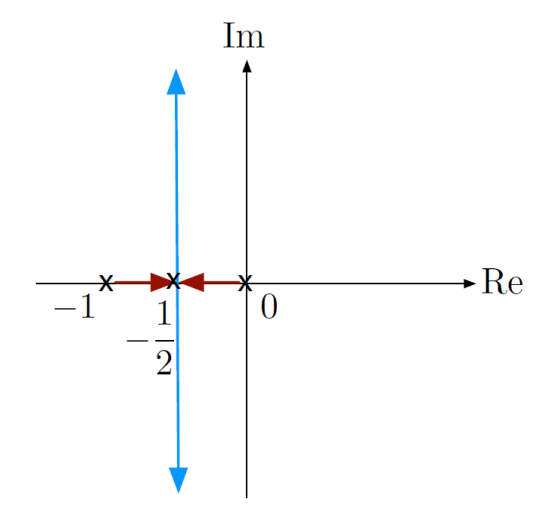
• We call $s=-\frac{1}{2}$ the point of breakaway from the real axis.

We can compare this plot to the admissible regions for given specs:

• $t_s\approx \frac{3}{\sigma }$ – We want $\sigma$ to be large. Recall that $s=-\sigma +j{\omega }_d$, so $\sigma =-\text{Re}(s)$, which means in this case we can only $\sigma =\frac{1}{2}$.
• $t_r\approx \frac{1.8}{{\omega }_n}$. We want ${\omega }_n$ to be large. Thus, we want a large $K$.
• $M_p$ – We want this to be inside the shaded; thus, we want a small $K$.

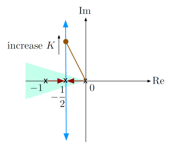
Thus, the root locus helps us visualize the trade-off between all the specs in terms of $K$.