Low-Order Approximations of High-Order Systems

It’s hard to find analytic formulas to evaluate the performance of high-order systems. Additional poles and zeroes far from the imaginary axis will have little impact on the settling time and other performance specifications. Good low-order approximations of a high-order system can be found by appropriately neglecting the less significant poles and zeros.

Time-Domain Response from Pole-Zero Plots

We can use pole-zero plots to help determine time-domain response of a system. The location of system poles determines the nature of the system’s response:

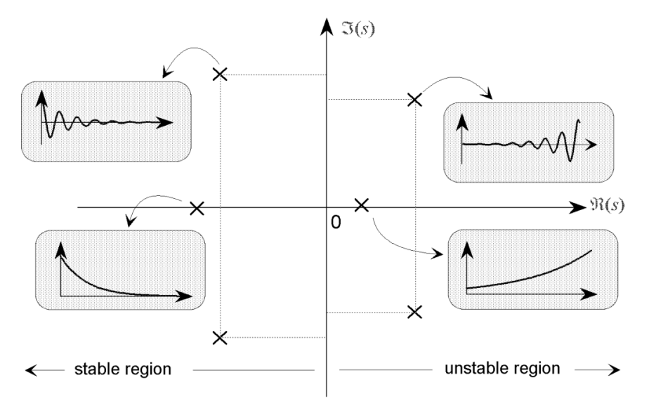
• Left-half plane ($\text{Re}(s)<0$) – Stable region
  • Real poles far from the left are fast-decaying exponentials
  • Real poles near origin are slow-decaying exponentials
  • Complex conjugate poles: Damped oscillations
• Right-half plane ($\text{Re}(s)>0$) – Unstable region
  • Real poles: Exponentially growing responses
  • Complex conjugate poles: Damped oscillations

Example

What’s the expected form of the response of a system with a pole-zero plot shown in the following Figure?

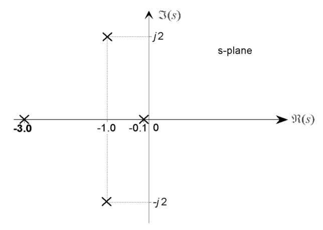
The system has four poles and no zeros. The two real poles correspond to decaying exponential terms $C_1{e}^{-3t}$ and $C_2{e}^{-0.1t}$, and the complex conjugate pole pair introduces an oscillatory component. $A{e}^{-t}\sin (2t+\varphi )$, so that the total homogeneous response is:

$$y_h(t)=C_1{e}^{-3t}+C_2{e}^{-0.1t}+A{e}^{-t}\sin (2t+\varphi )$$

• The term $e^{-3t}$ decays rapidly
• The term $e^{-0.1t}$ decays slowly. It is therefore the dominant long term response component in the overall homogeneous response.

For methods of approximation, see:

• Dominant Poles and Zeros
• Second-Order System Approximation