VAE Evidence Lower Bound

ELBO gives a lower bound on the log-likehood for VAE training:

$$\hat{\varphi }=\underset{\varphi }{\mathrm{argmax}}\left[\sum _{i=1}^I\log [Pr(x_i|\varphi )]\right]$$

where

$$Pr(x_i|\varphi )=\int {\text{Norm}}_{x_i}[f[z,\varphi ],{\sigma }^{2}I]\cdot {\text{Norm}}_z[0,I]dz$$

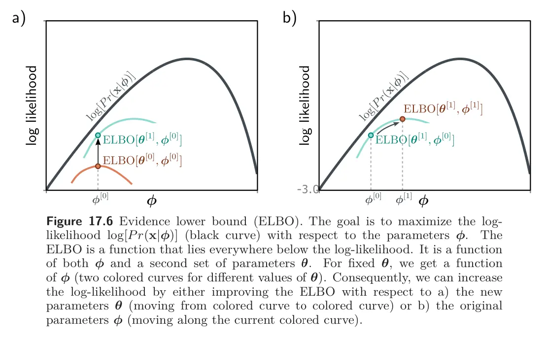
Specifically, ELBO is a function that is always less than or equal to the log-likelihood for a given value of $\varphi$, and will also depend on some other parameters $\theta$.

Jensen’s Inequality

To define this lower bound, we need Jensen’s Inequality for concave functions $g[\bullet ]$:

$$g[\mathbb{E}[y]]\ge \mathbb{E}[g[y]]$$

In this case, the concave function is the logarithm, so we have:

$$\log [\mathbb{E}[y]]\ge \mathbb{E}[\log [y]]$$

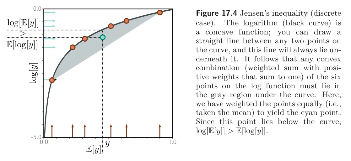
Writing out the expectation in full, we have:

$$\log \left[\int Pr(y)ydy\right]\ge \int Pr(y)\log [y]dy$$

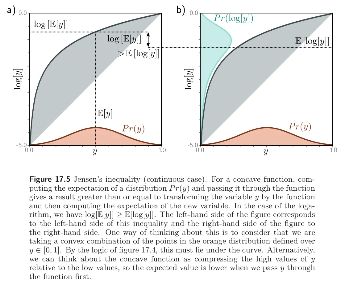
In fact, a slightly more general statement is true:

$$\log \left[\int Pr(y)h(y)dy\right]\ge \int Pr(y)\log [h[y]]dy$$

where $h[y]$ is a function of $y$. This follows because $h[y]$ is another random variable with a new distribution. Since we never specified $Pr(y)$, the relation remains true.

Derivation of the bound

We now use Jensen’s inequality to derive the lower bound for the log-likelihood. We start by introducing an arbitrary distribution $q(z)$ over the latent variables. Multiplying and dividing the log-likelihood by $q(z)$ lets us re-write the marginal likelihood as an expectation and apply Jensen’s inequality.

First:

$$\begin{array}{rl}\log [Pr(x|\varphi )]& =\log \left[\int Pr(x,z|\varphi )dz\right]\\ & =\log \left[\int q(z)\frac{Pr(x,z|\varphi )}{q(z)}dz\right]\end{array}$$

We then use Jensen’s inequality for the logarithm to find a lower bound:

$$\log \left[\int q(z)\frac{Pr(x,z|\varphi )}{q(z)}dz\right]\ge \int q(z)\log \left[\frac{Pr(x,z|\varphi )}{q(z)}\right]dz$$

where the right-hand side is termed the evidence lower bound or ELBO. It gets this name because $Pr(x|\varphi )$ is called the evidence in the context of Bayes’ rule.

In practice, the distribution $q(z)$ has parameters $\theta$, so the ELBO can be written as:

$$\text{ELBO}[\theta ,\varphi ]=\int q(z|\theta )\log \left[\frac{Pr(x,z|\varphi )}{q(z|\theta )}\right]dz$$

To learn the nonlinear latent variable model, we maximize this quantity as a function of both $\varphi$ and $\theta$. The neural architecture that computes this quantity is the VAE.

Properties

Let’s build some intuition about ELBO.

Consider that the original log-likelihood of the data is a function of the parameters $\varphi$ and that we want to find its maximum. For any fixed $\theta$, the ELBO is still a function of the parameters, but one that must lie below the original likelihood function.

• When we change $\theta$, we modify this function, and depending on our choice, the lower bound may move closer or further from the log-likelihood.
• When we change $\varphi$, we move along the lower bound function.

Tightness of the bound

The ELBO is tight when, for a fixed value of $\varphi$, the ELBO and the log-likelihood function coincide.

To find the distribution $q(z|\theta )$ that makes the bound tight, we factor the numerator of the log term in the ELBO using the definition of conditional probability:

$$\begin{array}{rl}\text{ELBO}[\theta ,\varphi ]& =\int q(z|\theta )\log \left[\frac{Pr(x,z|\varphi )}{q(z|\theta )}\right]dz\\ & =\int q(z|\theta )\log \left[\frac{Pr(z|x,\varphi )Pr(x|\varphi )}{q(z|\theta )}\right]dz\\ & =\int q(z|\theta )\log [Pr(x|\varphi )]dz+\int q(z|\theta )\log \left[\frac{Pr(z|x,\varphi )}{q(z|\theta )}\right]dz\\ & =\log [Pr(x|\varphi )]+\int q(z|\theta )\log \left[\frac{Pr(z|x,\varphi )}{q(z|\theta )}\right]dz\\ & =\log [Pr(x|\varphi )]-D_{KL}[q(z|\theta )||Pr(z|x,\varphi )]\end{array}$$

• The first integral disappears between lines 3 and 4 since $\log [Pr(x|\varphi )]$ does not depend on $z$, and the integral of the probability distribution $q(z|\theta )$ is one.
• In the last line, we used the definition of KL divergence.

This shows that the ELBO is the original log-likelihood minus the KL divergence $D_{KL}[q(z|\theta )||Pr(z|x,\varphi )]$. The KL divergence measures the “distance” between distributions and is always non-negative. Thus, it’s clear that the ELBO is a lower bound on $\log [Pr(x|\varphi )]$.

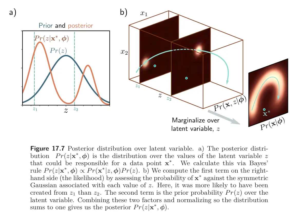
When $q(z|\theta )=Pr(z|x,\varphi )$, the KL distance will be zero, and the bound is tight. $Pr(z|x,\varphi )$ is the posterior distribution over the latent variables $z$ given observed data $x$; it indicates which values of the latent variable could have been responsible for the data point.

ELBO as reconstruction minus KL distance to prior

We have seen two ways to describe ELBO. A third way is to consider the bound as reconstruction error minus the distance to the prior:

$$\begin{array}{rl}\text{ELBO}& =\int q(z|\theta )\log \left[\frac{Pr(x,z|\varphi )}{q(z|\theta )}\right]dz\\ & =\int q(z|\theta )\log \left[\frac{Pr(x|z,\varphi )Pr(z)}{q(z|\theta )}\right]dz\\ & =\int q(z|\theta )\log [Pr(x|z,\varphi )]dz+\int q(z|\theta )\log \left[\frac{Pr(z)}{q(z|\theta )}\right]dz\\ & =\int q(z|\theta )\log [Pr(x|z,\varphi )]dz-D_{KL}[q(z|\theta )\left|\right|Pr(z)]\end{array}$$

• The joint distribution $Pr(x,z|\varphi )$ has been factored into conditional probability $Pr(x|z,\varphi )Pr(z)$ between the first and second lines
• The definition of KL divergence is used in the last line.

In this formulation:

1. The first term measures the average agreement $Pr(x|z,\varphi )$ of the latent variable and the data. This measures the reconstruction accuracy.
   • The $q(z|\theta )$ term identifies latents $z$ that might explain $x$. $Pr(x|z,\varphi )$ measures how much probability is assigned to the observed $z$ given $z$. The integral then averages this score over all possible $z$‘s.
2. The second term measures the degree to which the auxiliary distribution $q(z|\theta )$ matches the prior.

This formulation is the one that is used in the variational autoencoder.

While we initially introduced $q(z)$ as a mathematical tool, we now see that $q(z)$ has an important role in the tightness of ELBO, where the bound is tight when $q(z)=Pr(z|x,\varphi )$. We therefore choose a tractable parameterized distribution $q(z|x,\theta )$ (usually a multivariate normal distribution) and optimize it as an approximation to the generally intractable $Pr(z|x,\varphi )$. This approximation is called the variational posterior.