GAN Stability Analysis

Theoretically, the GAN is fairly straightforward. However, they are notoriously difficult to train.

• For example, to get DCGAN to train reliable, they had to use strided convolutions for upsampling and downsampling, use BatchNorm in both the generator and discriminator except in the last and first layers, use leaky ReLU in the discriminator, use Adam but with a lower momentum coefficient.
• This instability is unusual; many deep learning models are relatively robust to such choices.

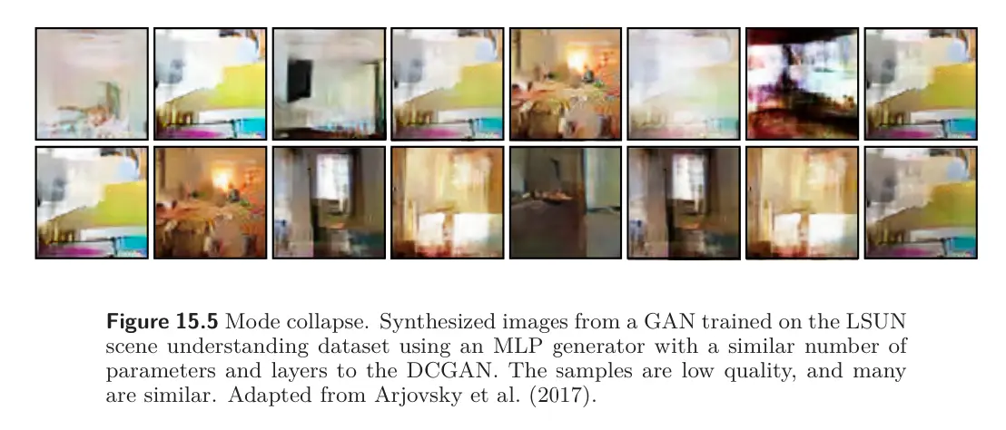
A common failure mode is that the generator makes plausible samples, but only representing a subset of the data. This is known as mode dropping. An extreme version of this phenomenon can occur where the generator entirely or mostly ignores the latent variable $z$ and collapses all samples to one or a few points; this is known as mode collapse.

Loss function analysis

To understand why GANs are difficult to train, it’s necessary to understand what the loss function represents. Recall that we can write the GAN objective as two loss functions:

$$\begin{array}{rl}L[\varphi ]& =\sum _j-\log [1-\text{sig}[f[g[z_j,\theta ],\varphi ]]]-\sum _i\log [\text{sig}[f[x_i,\varphi ]]]\\ L[\theta ]& =\sum _j\log [1-\text{sig}[f[g[z_j,\theta ],\varphi ]]]\end{array}$$

where the first loss function trains the discriminator and the second loss function trains the generator.

If we divide the two sums in the first line by the numbers $I,J$ of real and generated samples, then the loss function can be written in terms of expectations:

$$\begin{array}{rl}L[\varphi ]& =-\frac{1}{J}\sum _{j=1}^J\left(\log \right[1-\text{sig}[f[g[z_j,\theta ],\varphi ]]\left]\right)-\frac{1}{I}\sum _{i=1}^I\left(\log \right[\text{sig}[f[x_i,\varphi ]]\left]\right)\\ & \approx {\mathbf{E}}_{x^{\ast }}\left[\log \right[1-\text{sig}[f[x^{\ast },\varphi ]]\left]\right]-{\mathbb{E}}_x\left[\log \right[\text{sig}[f[x,\varphi ]]\left]\right]\\ & =-\int Pr(x^{\ast })\log [1-\text{sig}[f[x^{\ast },\varphi ]]]dx-\int Pr(x)\log [\text{sig}[f[x,\varphi ]]]dx\end{array}$$

where $Pr(x^{\ast })$ is the probability distribution over the generated samples, and $Pr(x)$ is the true probability distribution over the samples.

When $I=J$, the optimal discriminator for an example $\tilde{x}$ of unknown origin is:

$$Pr(\text{real}|\tilde{x})=\text{sig}[f[\tilde{x},\varphi ]]=\frac{Pr(\tilde{x}|\text{real})}{Pr(\tilde{x}|\text{generated})+\text{Pr}(\tilde{x}|\text{real})}=\frac{Pr(x)}{Pr(x^{\ast })+Pr(x)}$$

where on the right side, we evaluate $\tilde{x}$ against the generated distribution $Pr(x^{\ast })$ and the real distribution $Pr(x)$. Substituting this back into our loss functoin:

$$\begin{array}{rl}L[\varphi ]& =-\int Pr(x^{\ast })\log [1-\text{sig}[f[x^{\ast },\varphi ]]]dx-\int Pr(x)\log [\text{sig}[f[x,\varphi ]]]dx\\ & =-\int Pr(x^{\ast })\log \left[1-\frac{Pr(x)}{Pr(x^{\ast })+Pr(x)}\right]d{x}^{\ast }-\int Pr(x)\log \left[\frac{Pr(x)}{Pr(x^{\ast })+Pr(x)}\right]dx\\ & =-\int Pr(x^{\ast })\log \left[\frac{Pr(x^{\ast })}{Pr(x^{\ast })+Pr(x)}\right]d{x}^{\ast }-\int Pr(x)\log \left[\frac{Pr(x)}{Pr(x^{\ast })+Pr(x)}\right]dx\end{array}$$

Disregarding additive and multiplicative constants, this is the Jensen-Shannon divergence between the synthesized distribution $Pr(x^{\ast })$ and the true distribution $Pr(x)$:

$$\begin{array}{rl}{D}_{JS}[& Pr(x^{\ast })||Pr(x)]\\ & =\frac{1}{2}{D}_{KL}\left[Pr(x^{\ast })\left|\right|\frac{Pr(x^{\ast })+Pr(x)}{2}\right]+\frac{1}{2}{D}_{KL}\left[Pr(x)\left|\right|\frac{Pr(x^{\ast })+Pr(x)}{2}\right]\\ & =\frac{1}{2}\int \underset{\text{quality}}{\underbrace{Pr(x^{\ast })\log \left[\frac{2Pr(x^{\ast })}{Pr(x^{\ast })+Pr(x)}\right]d{x}^{\ast }}}+\frac{1}{2}\int \underset{\text{coverage}}{\underbrace{Pr(x)\log \left[\frac{2Pr(x)}{Pr(x^{\ast })+Pr(x)}\right]dx}}\end{array}$$

where $D_{KL}[\bullet \mid \mid \bullet ]$ is the KL divergence.

The first term indicates the distance will be small if, wherever the sample density $Pr(x^{\ast })$ is high, the mixture $(Pr(x^{\ast })+Pr(x))/2$ has high probability. In other words, it penalizes regions with samples $x^{\ast }$ but no real examples $x$; it enforces the quality of generated samples.

The second term says that the distance will be small if, wherever the true density $Pr(x)$ is high, the mixture $(Pr(x^{\ast })+Pr(x))/2$ has high probability. In other words, it penalizes regions with real examples but no generated samples. This enforces coverage.

We can see that the second term does not depend on the generator parameters $\varphi$; consequently, the generator doesn’t care much about coverage, though it is still implicitly included through $Pr(x^{\ast })$. It is happy to generate a subset of possible examples accurately. This is the likely reason for mode dropping/collapse.

Vanishing gradients

We saw that when the discriminator is optimal, the loss function maximizes a measure of the distance between the generated and real samples. However, there’s a problem with using this distance between probability distributions as the criterion for optimizing GANs. If the probability distributions are completely disjoint, this distance is infinite, and any small change to the generator will not decrease the loss. The same phenomenon can be seen when we consider the original formulation; if the discriminator can perfectly separate the generated and real samples, no small change to the generated data will change classification score.

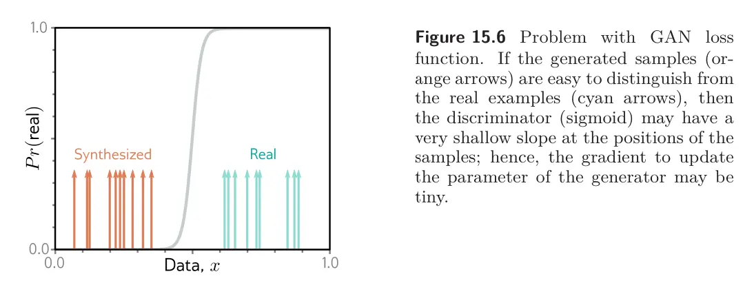
Unfortunately, the distributions may really be disjoint; the generated samples lie in a subspace that is the size of the latent variable $z$, and the real examples also lie in a low-dimension al subspace due to the physical processes that created the data. There may be very little or no overlap between these two subspaces, and the result is very small or no gradients.

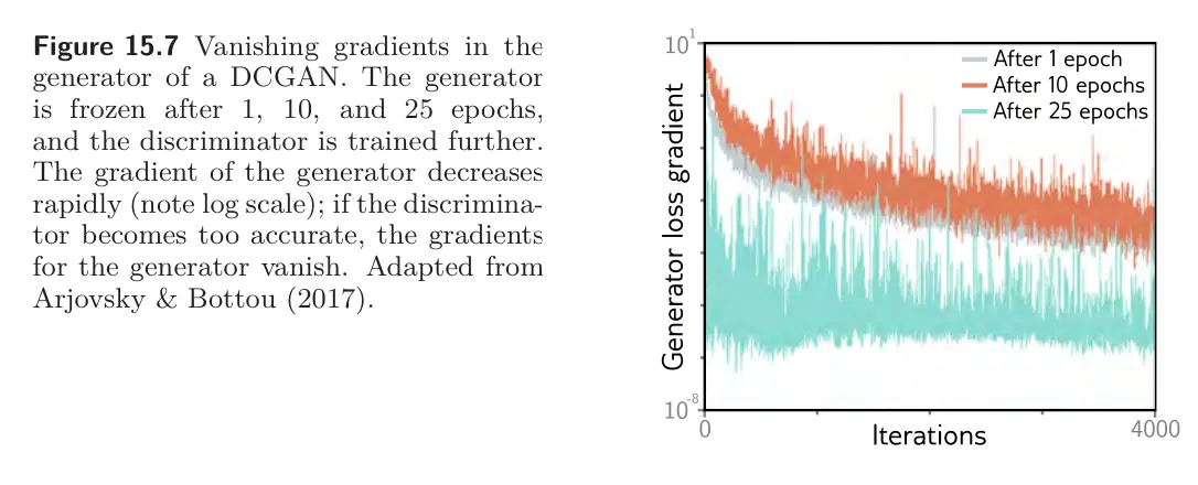
We can see an empirical version of this below. If the DCGAN generator is frozen and the discriminator is updated repeatedly so that its classification performance improves, the generator gradients decrease. In short, there is a very fine balance between the quality of the discriminator and the generator; if the discriminator becomes too good, the training updates of the generator are attenuated.

dl
Why are GANs hard to train?
?

1. Training is a coupled, non-stationary game: updating either network changes the objective faced by the other.
2. With an optimal discriminator, the original GAN objective corresponds to minimizing the Jensen–Shannon divergence between the real and generated distributions. If they have little or no overlap, the discriminator sigmoid can saturate, giving the generator vanishing gradients.

+++