Linear Regression as MLE

Regression problems can be expressed in terms of error minimization, such as Ordinary Least Squares. We can also view it as a probabilistic maximum likelihood estimation problem.

The goal in the regression problem is to make predictions for the target variable $t$ given some new value of the input variable $x$. This is done by using a set of training data comprising $N$ input values, $\mathbf{x}=(x_1,\dots ,x_N)$ and their corresponding values $\mathbf{t}=(t_1,\dots ,t_N)$.

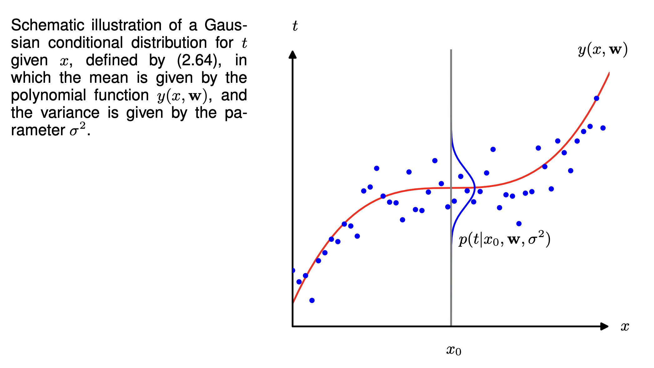
We can express our uncertainty over the value of the target variable using a probability distribution. Given a value of $x$, the corresponding $t$ has a Gaussian distribution with a variance ${\sigma }^2$, and a mean equal to $y(x,\mathbf{w})$, such that:

$$\begin{array}{rl}y(x,\mathbf{w})& =w_0+w_{1}x+w_2{x}^2+\cdots +w_M{x}^M\\ & =\sum _{j=0}^M{w}_j{x}^j\end{array}$$

Thus, we have:

$$p(t|x,\mathbf{w},{\sigma }^2)=\mathcal{N}(t|y(x,\mathbf{w}),{\sigma }^2)$$

This is shown in the diagram below. Instead of predicting a point with the function $y(x,\mathbf{w})$, we’re predicting a distribution where $y(x,\mathbf{w})$ is the mean.

We can then use our training data $\mathbf{x}$ and labels $\mathbf{t}$ to determine the values of the unknown parameters $\mathbf{w}$ and ${\sigma }^2$ by maximum likelihood. If the data is drawn independently the distribution, the likelihood function is:

$$p(\mathbf{t}|\mathbf{x},\mathbf{w},{\sigma }^2)=\prod _{n=1}^N\mathcal{N}(t_n|y(x_n,\mathbf{w}),{\sigma }^2)$$

Like our Gaussian MLE example, we can maximize the logarithm of the likelihood function:

$$\ln p(\mathbf{t}|\mathbf{x},\mathbf{w},{\sigma }^2)=-\frac{1}{2{\sigma }^2}\sum _{n=1}^N\{y(x_n,\mathbf{w})-t_n\}-\frac{N}{2}\ln {\sigma }^2-\frac{N}{2}\ln (2\pi )$$

Now, we would want to maximize the above expression with respect to $\mathbf{w}$:

• We can ignore the 2nd and 3rd term because they don’t depend on $\mathbf{w}$.
• Scaling the log likelihood by a positive constant coefficient doesn’t change the location of the maximum with respect to $\mathbf{w}$, so we can replace $1/2{\sigma }^2$ with just $1/2$.
• Minimizing the negative log likelihood is equivalent to maximizing the log likelihood.

Thus, our MLE is equivalent, as far as $\mathbf{w}$ is concerned, to minimizing the sum-of-squares error defined by:

$$E(\mathbf{w})=\frac{1}{2}\sum _{n=1}^N\{y(x_n,\omega )-t_n{\}}^2$$

(The square is added to guarantee positive values).

Thus, we’ve shown how the sum-of-squares error function arises as a consequence of maximizing the likelihood under the assumption of a Gaussian noise distribution.

We can also use maximum likelihood to determine ${\sigma }^2$. Maximizing the logarithm of the likelihood function with respect to ${\sigma }^2$ gives:

$${\sigma }_{\text{ML}}^2=\frac{1}{N}\sum _{n=1}^N\{y(x_n,{\mathbf{w}}_{\text{ML}})-t_n{\}}^2$$

We can first determine the parameter vector ${\mathbf{w}}_{\text{ML}}$ governing the mean, and subsequently use this to find the variance ${\sigma }_{\text{ML}}^2$ as was the case for the Gaussian MLE.

Since we have determined the parameters $\mathbf{w}$ and ${\sigma }^2$, we can now make predictions for new values of $x$. Our model is probabilistic, so these are expressed in terms of the predictive distribution that gives the probability distribution over $t$, rather than simply a point estimate. These distributions can be obtained by substituting the maximum likelihood parameters into our original distribution expression to get:

$$p(t|x,{\mathbf{w}}_{\text{ML}},{\sigma }_{\text{ML}}^2)=\mathcal{N}(t|y(x,{\mathbf{w}}_{\text{ML}}),{\sigma }^2)$$