1D Kalman Filter with Process Noise

In the real world, there are uncertainties in the system dynamic model. Just because we assume something should be constant, like the resistance of a resistor, doesn’t mean it’s actually constant – the resistant may change slightly due to environmental changes.

This uncertainty of the system model is called Process Noise. The process noise produces estimation errors.

The Process Noise Variance is denoted by the letter $q$.

For a constant system, the Covariance Extrapolation/Prediction Equation for constant dynamics would be:

$${\hat{p}}_{n+1,n}=p_{n,n}+q_n$$

Kalman Filter Equations

Thus, we have the following updated Kalman Filter equations in 1D:

State and Covariance Update

$$\begin{array}{rl}{\hat{x}}_{n,n}& ={\hat{x}}_{n,n-1}+K_n(z_n-{\hat{x}}_{n,n})\\ p_{n,n}& =(1-K_n)p_{n,n-1}\\ K_n& =\frac{p_{n,n-1}}{p_{n,n-1}+r_n}\end{array}$$

State and Covariance Predict

State

Constant system dynamics:

$$\begin{array}{r}{\hat{x}}_{n+1,n}={\hat{x}}_{n,n}\end{array}$$

Constant velocity:

$$\begin{array}{rl}{\hat{x}}_{n+1,n}& ={\hat{x}}_{n,n}+\Delta t{\hat{\dot{x}}}_{n,n}\\ {\hat{\dot{x}}}_{n+1,n}& ={\hat{\dot{x}}}_{n,n}\end{array}$$

Covariance

Constant system dynamics:

$$p_{n+1,n}^x=p_{n,n}^x+q_n$$

Constant velocity:

$$\begin{array}{rl}{p}_{n+1,n}^x& =p_{n,n}^x+\Delta t^2{p}_{n,n}^v\\ p_{n+1,n}^v& =p_{n,n}^v+q_n\end{array}$$

Example: Temperature Estimation

We want to estimate the temperature of the liquid in a tank.

We assume that at a steady state, the liquid temperature is constant. However, some fluctuations in the true liquid temperature are possible. The system can be described with:

$$x_n=T+w_n$$

where:

• $T$ is the constant temperature
• $w_n$ is a random process noise with variance $q$

Given info:

• Let’s assume a true temperature of 50 degrees.
• We assume the model is accurate, so we set the process noise variance $q$ to $0.0001$.
• The measurement error (standard deviation) is 0.1 degrees Celsius.
• The measurements are taken every 5 seconds.
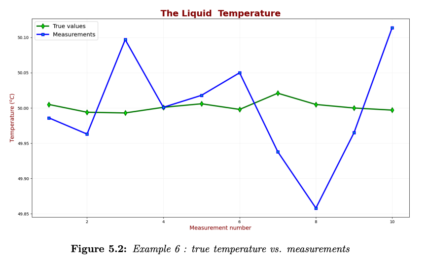
• The true liquid temperature values at the measurement points are: 50.005, 49.994, 49.993, 50.001, 50.006, 49.998, 50.021, 50.005, 50, and 49.997
• The measurements are: 49.986, 49.963, 50.09, 50.001, 50.018, 50.05, 49.938, 49.858, 49.965, and 50.114

The following chart compares the true liquid temperature and the measurements:

Iteration 0

Before the first iteration, we initialize the Kalman Filter and predict the following state.

We start with a guess of $60°C$. Our guess is imprecise, so we set our initialization estimate error $\sigma$ to a large value of $100$. Then, the estimate variance of the initialization is the error variance ${\sigma }^2$:

$$p_{0,0}=100^2=10,000$$

Prediction: Since our model has constant dynamics, the predicted estimate is equal to the current estimate:

$${\hat{x}}_{1,0}=60°C$$

The extrapolated estimate variance:

$$p_{1,0}=p_{0,0}+q=10000+0.0001=10000.0001$$

Iteration 1

Measure: We get a measurement value of

$$z_1=49.986°C$$

Since the measurement error is $\sigma =0.1$, the variance is ${\sigma }^2=0.01$. Thus, the measurement variance is:

$$r_1=0.01$$

Update: The Kalman Gain is

$$K_n=\frac{p_{1,0}}{p_{1,0}+r_1}=\frac{10000.0001}{10000.0001+0.01}=0.999999$$

A Kalman Gain of 1 means that rur estimate error is much bigger than our measurement error, so our update will almost completely disregard the previous prediction and just use the measurement.

Estimating the current state:

$$\begin{array}{rl}{\hat{x}}_{1,1}& ={\hat{x}}_{1,0}+K(z_1-{\hat{x}}_{1,0})\\ & =60+0.999999(49.986-60)\\ & =49.986°C\end{array}$$

Updating the current estimate variance:

$$\begin{array}{rl}{p}_{1,1}& =(1-K_1)p_{1,0}\\ & =(1-0.999999)10000.0001\\ & =0.01\end{array}$$

Predict: Since our system’s dynamic model is constant (the liquid temperature doesn’t change), we have

$${\hat{x}}_{2,1}={\hat{x}}_{1,1}=49.986°C$$

The extrapolated estimate variance is

$$p_{2,1}=p_{1,1}+q=0.01+0.0001=0.0101$$

Iteration 2

The second measurement is

$$z_2=49.963°C$$

Since the measurement error is $\sigma =0.1$, the variance is ${\sigma }^2=0.01$. Thus, the measurement variance is

$$r_2=0.01$$

Update: Kalman Gain calculation gives us

$$K_2=\frac{p_{2,1}}{p_{2,1}+r_2}=\frac{0.0101}{0.0101+0.01}=0.50$$

The Kalman Gain is around $0.5$, so the weight of the estimate and the measurement weight are basically equal.

Estimating the current state:

$$\begin{array}{rl}{\hat{x}}_{2,2}& ={\hat{x}}_{2,1}+K_2(z_2-x_{2,1})\\ & =50.13+0.5(48.44-50.13)=49.33\end{array}$$

Updating the current estimate variance:

$$p_{2,2}=(1-K_2)p_{2,1}=(1-0.5)0.0101=0.005$$

Predict: Since our system’s dynamic model is constant (the liquid temperature doesn’t change), we have

$${\hat{x}}_{3,2}={\hat{x}}_{2,2}=49.33°C$$

The extrapolated estimate variance is

$$p_{3,2}=p_{2,2}+q=0.005+0.0001=0.0051$$

Results & Analysis

After 10 iterations, we plot the Kalman Gain:

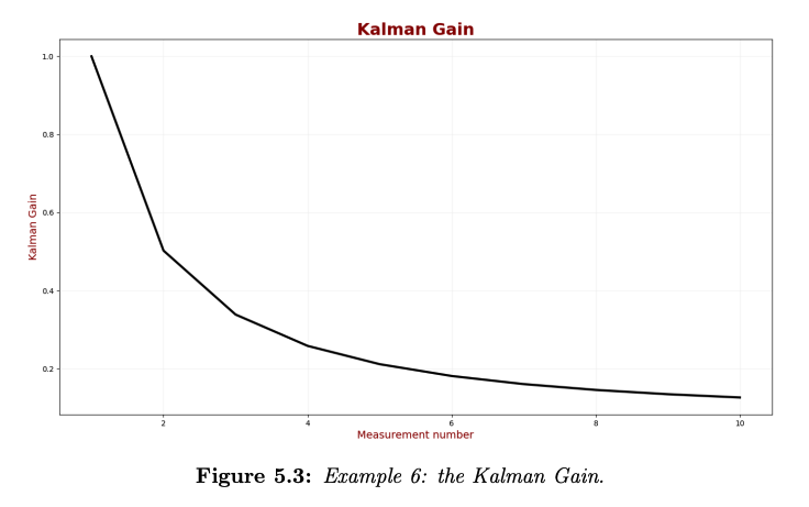
As we can see, the Kalman Gain gradually decreases; therefore, the KF converges.

The following chart compares the true value, measured values, and estimates. The confidence interval is $95\%$.

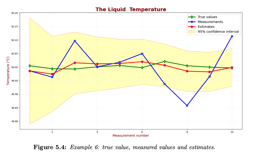
As you can see, the estimated value converges toward the true value. The KF estimates uncertainties are too high for the 95% confidence level. The yellow area is too broad; the KF is too conservative, thinking that its uncertainty is higher than it actually is, despite the fact that the estimates appear to track the true values fairly well.

Example (Failed): Increasing Liquid Temperature

We want to estimate the temperature of the liquid in the tank. In this case, the dynamic model of the system is not constant – the liquid is heating at a rate of $0.1°C$ per second.

The Kalman Filter parameters are similar to the previous example:

• We assume that the model is accurate; the process noise variance $q$ is set to $0.0001$
• The measurement error (standard deviation) is $0.1°C$.
• The measurements are taken every 5 seconds.
• The dynamic model of the system is constant.

Let’s say that:

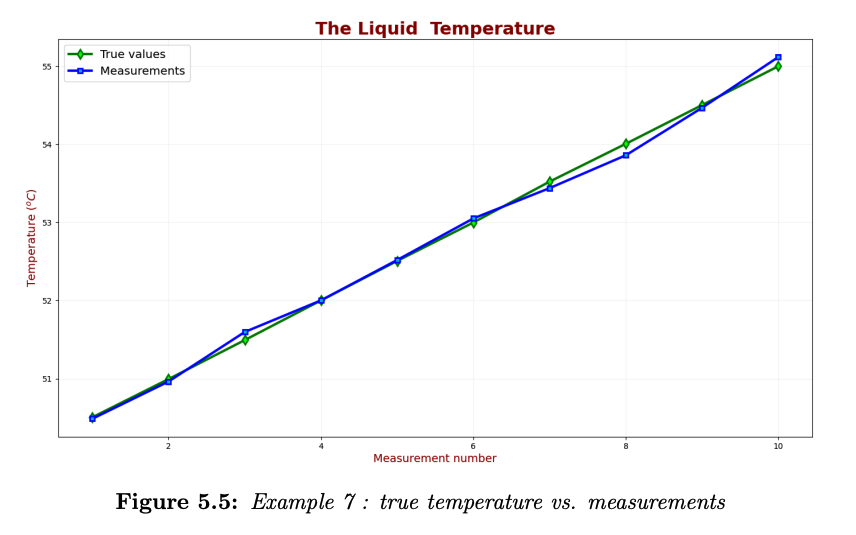
• The true liquid temperatures are: 50.505, 50.994, 51.493, 52.001, 52.506, 52.998, 53.521, 54.005, 54.5, and 54.997.
• The measurements are: 50.486, 50.963, 51.597, 52.001, 52.518, 53.05, 53.438, 53.858, 54.465, and 55.114.

The following chart compares the true liquid temperature and the measurements:

Iteration 0

Before the first iteration, we must initialize the Kalman Filter and predict the following state (which is the first state).

Initialization: We don’t know the true temperature of the liquid in a tank, and our guess is $10°C$:

$${\hat{x}}_{0,0}=10°C$$

Our guess is imprecise, so we set our initialization estimate error $\sigma$ to 100. The estimate variance of the initialization is the error variance, ${\sigma }^2$:

$$p_{0,0}=100^2=10,000$$

Prediction: We predict the next state based on the initialization values. Since our model has constant dynamics, the predicted estimate is equal to the current estimate:

$${\hat{x}}_{1,0}=10°C$$

The predicted estimate variance:

$$p_{1,0}=p_{0,0}+q=10000+0.0001=10000.0001$$

Results

The following chart compares the true value, measured values and estimates over 10 iterations:

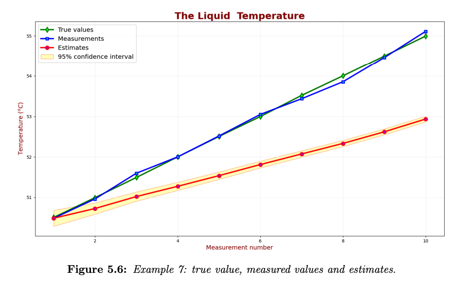
As we can see, the Kalman Filter has failed to provide a reliable estimation. There is a lag error. There are two reasons for the lag error here:

• The dynamic model doesn’t fit the case. The dynamic model heats up by 0.25 degrees per unit time, while in reality it’s more 0.5 degrees.
• We have chosen very low process noise $q=0.0001$, while the true temperature fluctuations are much more significant.
• Another problem is a low estimate uncertainty. The KF failed to provide accurate estimates and is also confident in its estimates. This is an example of a bad KF design.

There are two ways to fix the lag error:

• If we know that the liquid temperature can change linearly, we can define a new model that considers a possible linear change in the liquid temperature. We did this in Example 4. This method is preferred. However, this method won’t improve the Kalman Filter performance if the temperature change can’t be modeled.
• On the other hand, since our model is not well defined, we can adjust the process model reliability by increasing the process noise ($q$). See the next example for details.

Example (Good): Increasing Liquid Temperature

This example is similar to the previous example, with only one change. Since our process is not well-defined, we increase the process variance $q$ to $0.15$.

Iteration 0

Initialization: We don’t know the true temperature of the liquid in a tank, and our guess is

$${\hat{x}}_{0,0}=10°C$$

Prediction: Now we predict the next state based on the initialization values

$${\hat{x}}_{1,0}=10°C$$

The extrapolated estimate variance:

$$p_{1,0}=p_{0,0}+q=10000+0.15=10000.15$$

Results

The following chart compares the true value, measured values, and estimates.

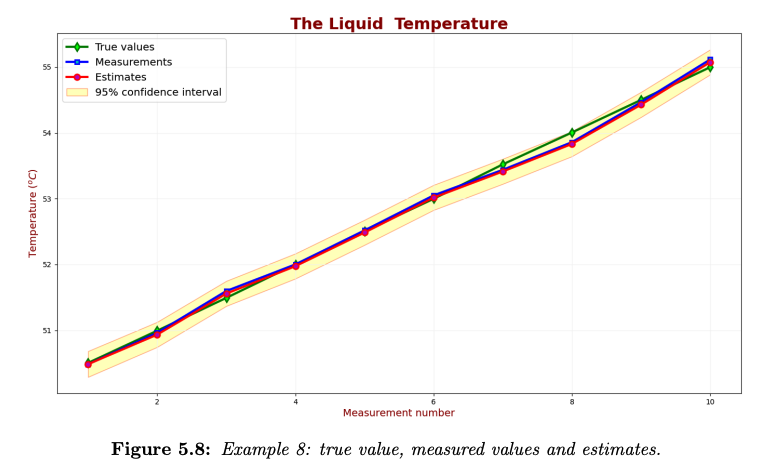
As you can see, the estimates following the measurements. There is no lag error.

Let’s take a look at the Kalman Gain:

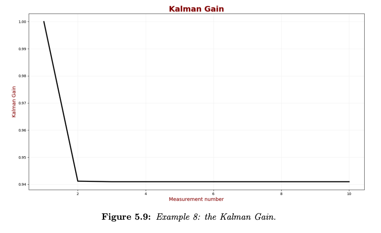
Due to the high process uncertainty, the measurement weight is much higher than the weight of the estimate. Thus, the Kalman Gain is high, and it converges to 0.94.

The good news is we can trust the estimates of this KF. The true values are within the 95% confidence region.zkz