Infinite-horizon MDP Solutions

It’s more common for the actual horizon of a problem to be unknown. If we tried to take our definition of $Q^h$ from Finite-horizon MDP Solutions and set $h=\infty$, $Q^{\infty }$ values for all actions could be infinite, and there would be no way to select one over the other.

There are 2 standard ways to deal with this problem:

• Take the average over all time-steps
• Take a discounted infinite horizon.

In the discounted infinite horizon, we select a discount factor $0<\gamma <1$. On each step, our life might with a probability of $1-\gamma$, giving us an expected lifetime of $1/(1-\gamma )$. Unlike Finite-horizon MDP Solutions, we don’t need a different policy for a different horizon; if we survive today, our expected future lifetime is just as long as yesterday.

Instead of trying to find a policy that maximizes expected finite-horizon undiscounted value,

$$\mathbf{E}\left[\sum _{t=0}^h{R}_t|\pi ,s_0\right]$$

we will try to find one that maximizes infinite-horizon discounted value:

$$\mathbf{E}\left[\sum _{t=0}^{\infty }{\gamma }^t{R}_t|\pi ,s_0\right]=\mathbf{E}[R_0+\gamma R_1+{\gamma }^2{R}_2+\dots |\pi ,s_0]$$

Unlike finite-horizon and it’s use of $h$ (horizon), the $t$ indices here are not the number of steps to go, but the number of steps forward from the starting state (there is no notion of “steps to go” in the infinite horizon case).

Why do we do discounting? Two reasons:

• In economic terms, you’d generally rather have some money today than that same amount of money next week (because you could use it now or invest it).
• Think of the whole process terminating, with probability 1 − γ on each step of the interaction. This value is the expected amount of reward the agent would gain under this terminating model.

Finding an optimal policy

The best way of behaving in an infinite-horizon discounted MDP is not time-dependent. At every step, your expected future lifetime, given that you have survived until now, is $1/(1-\gamma )$.

An important theorem about MDPs is: there exists a stationary optimal policy ${\pi }^{\ast }$ (there may be more than one) such that for all $s\in S$ and all other policies $\pi$, we have

$$V_{{\pi }^{\ast }}(s)\ge V_{\pi }(s)$$

Value iteration

Define $Q^{\ast }(s,a)$ to be expected infinite-horizon discounted value of being in state s, executing action a, and executing an optimal policy ${\pi }^{\ast }$ thereafter. Using similar reasoning the recursive definition of $V_{\pi }$ (see Policy Evaluation), we can express this value recursively as

$$Q^{\ast }(s,a)=R(s,a)+\gamma \sum _{s^{\prime }}T(s,a,s^{\prime })\underset{a^{\prime }}{\max }{Q}^{\ast }(s^{\prime },a^{\prime })$$

This is also a set of equations, one for each $(s,a)$ pair. If we knew the optimal action-value function, then we could derive an optimal policy ${\pi }^{\ast }$ as

$${\pi }^{\ast }(s)={\text{argmax}}_{a^{\prime }}{Q}^{\ast }(s,a)$$

We can iteratively solve for the $Q^{\ast }$ values with the value iteration algorithm:

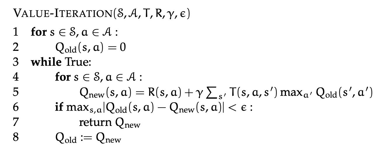
This is essentially just executing the above equation over and over again until we converge to optimal $Q$-values! Super simple.

Value Iteration Theory

There are a lot of nice theoretical results about value iteration. For some given (not necessarily optimal) $Q$ function, define ${\pi }_Q(s)={\text{argmax}}_{a}Q(s,a)$.

• After executing value iteration with parameter $ϵ$, $||V_{{\pi }_{Q\text{new}}}-V_{{\pi }^{\ast }}|{|}_{\text{max}}<ϵ$.
• There is a value of $ϵ$ such that

$$||Q_{\text{old}}-Q_{\text{new}}|{|}_{\text{max}}<ϵ⟹{\pi }_{Q_{\text{new}}}={\pi }^{\ast }$$

• As the algorithm executes, $||V_{{\pi }_{Q_{\text{new}}}}-V_{{\pi }^{\ast }}|{|}_{\text{max}}$ decreases monotonically on each iteration
• The algorithm can be executed asynchronously, in parallel: as long as all $(s,a)$ pairs are updated infinitely often in an infinite run, it still converges to optimal value.