CNN Architecture

Here is the form of a typical convolutional network:

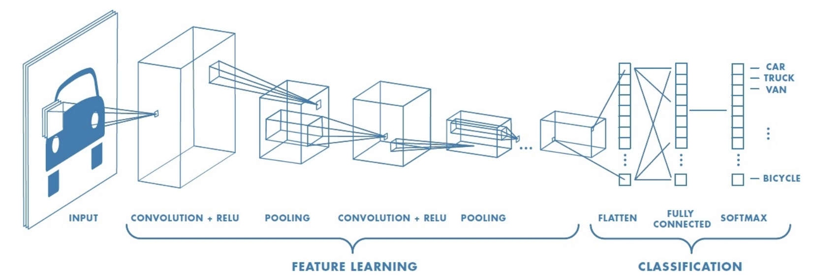
Generally:

• Each Convolution Layer is accompanied by a ReLU layer
• Usually there are multiple filter/ReLU layers, then a max pooling layer, then some more filter/ReLU layers, then max pooling again
• Once the output is down to a relatively small size, there is typically a last fully-connected layer, leading into an Activation Function such as softmax that produce the final output.

The exact design of these structures is an art—there is not currently any clear theoretical (or even systematic empirical) understanding of how these various design choices affect overall performance of the network.

The critical point for us is that this is all just a big neural network, which takes an input and computes an output. The mapping is a differentiable function of the weights, which means we can adjust the weights to decrease the loss by performing gradient descent, and we can compute the relevant gradients using backpropagation.

Backpropagation Example

Let’s work through a very simple example of how back-propagation can work on a convolutional network. The architecture is shown below.

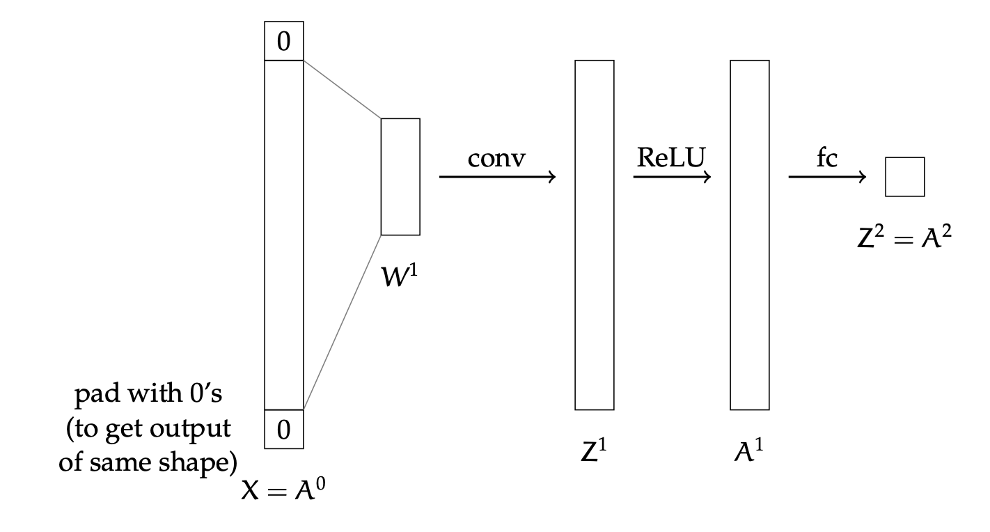
Assume we have a one-dimensional single-channel image, of size $n\times 1\times 1$ and a single $k\times 1\times 1$ filter (where we omit the filter bias) in the first convolutional layer. Then we pass it through a ReLU layer and a fully-connected layer with no additional activation function on the output.

For simplicity, assume $k$ is odd. Let the input image $X=A^0$, and assume we are using squared loss. Then we can describe the forward pass as follows:

$$\begin{array}{rl}{Z}_i^l& =W^{1^T}\cdot A_{[i-\lfloor k/2\rfloor :1+\lfloor k/2\rfloor ]}^0\\ A^1& =\text{ReLU}(Z^1)\\ A^2& =W^{2^T}{A}^1\\ L(A^2,y)& =(A^2-y{)}^2\end{array}$$

How do we update the weights in filter $W^1$?

$$\frac{\partial \text{ loss}}{\partial W^1}=\frac{\partial Z^1}{\partial W^1}\cdot \frac{\partial A^1}{\partial Z^1}\cdot \frac{\partial \text{ loss}}{\partial A^1}$$

We have:

• $\partial Z^1/\partial W^1$ is the $k\times n$ matrix such that $\partial Z_i^l/\partial W_j^1=X_{i-\lfloor k/2\rfloor +j-1}$.
  • So, for example, if $i=10$, which corresponds to column 10 in this matrix, which illustrates the dependence of pixel 10 of the output image on the weights, and if $k=5$, then the elements in column 10 will be $X_8,X_9,X_{10},X_{11},X_{12}$.
• $\partial A^1/\partial Z^1$ is the $n\times n$ diagonal matrix such that:

$$\partial A_i^1/\partial Z_i^1=\{\begin{array}{ll}1& \text{if }{Z}_i^1>0\\ 0& \text{otherwise}\end{array}$$

• $\partial \text{ loss}/\partial A^1=\partial \text{ loss}/\partial A^2\cdot \partial A^2/\partial A^1=2(A^2-y)W^2$
  • This is an $n\times 1$ vector

Multiplying these components together gives us the desired gradient, with dimensions $k\times 1$.