Divide and Conquer Recurrences

Typical divide-and-conquer algorithms break a given problem into $a$ smaller pieces, each of which is of size $n/b$. It then spends $f(n)$ time to combine these subproblem solutions into a complete result.

Let $T(n)$ denotes the worst-case time this algorithm takes to solve a problem of size $n$. Then, $T(n)$ is given by the following recurrence relation:

$$T(n)=a\cdot T(n/b)+f(n)$$

Consider the following examples of this:

• Mergesort – The running time of mergesort is governed by the recurrence $T(n)=2T(n/2)+O(n)$. The algorithm divides the data into 2 sub-problems of equal size, and then spends linear time merging the halves after they are sorted. This recurrence evaluates to $T(n)=O(n\lg n)$.
• Binary Search – The running time of binary search is governed by the recurrence $T(n)=T(n/2)+O(1)$. At each step we spend constant time to reduce the problem to 1 sub-problem that is half its size. This recurrence evaluates to $T(n)=O(\lg n)$.
• Fast heap construction – The “bubble down” method of heap construction builds an $n$-element heap by constructing two $n/2$ element heaps and then merging them with the root in logarithmic time. The running time is thus governed by the recurrence relation $T(n)=2T(n/2)+O(\lg n)$. This recurrence evaluates to $T(n)=O(n)$.

Solving a recurrence means finding a nice closed form describing or bounding the result. We can use the master theorem to solve the recurrence relations typically arising from divide-and-conquer algorithms.

Solving Divide-and-Conquer Recurrences

Divide-and-conquer recurrences of the form $T(n)=aT(n/b)+f(n)$ are generally easy to solve, because the solutions fall into three distinct cases:

1. If $f(n)=O(n^{{\log }_{b}a-ϵ})$ for some constant $ϵ>0$, then $T(n)=\Theta (n^{{\log }_{b}a})$.
2. If $f(n)=\Theta (n^{{\log }_{b}a})$, then $T(n)=\Theta (n^{{\log }_{b}a}\lg n)$.
3. If $f(n)=\Omega (n^{{\log }_{b}a+ϵ})$ for some constant $ϵ>0$, and if $af(n/b)\le cf(n)$ for some $c<1$, then $T(n)=\Theta (f(n))$.

The above is called the master theorem.

The figure below shows the recursion tree associated with a typical $T(n)=aT(n/b)+f(n)$ divide-and-conquer algorithm.

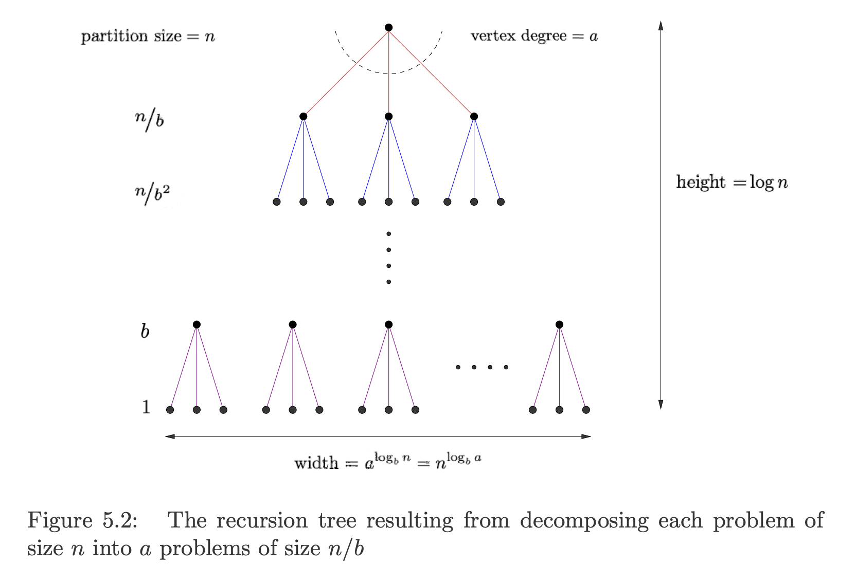
Each problem of size $n$ is decomposed into sub-problems of size $n/b$.

Each subproblem of size $k$ takes $O(f(k))$ time to deal with internally; there is an internal evaluation cost at each level of the recursion.

• This includes the work done outside of the recursive calls, such as dividing the problem, processing the subproblems (e.g., partitioning in quicksort), and combining or merging the results (e.g., merging in mergesort).
• At the root, the subproblem size is $k=n$ (where $n$ is used to denote the size of the original problem), but as we go down the tree, we have $k=n/b^2$, $k=n/b^3$, etc.

Note on notation: Why do we use $T(n)=a\cdot T(n/b)+f(n)$ instead of $f(k)$? This recurrence relation describes the total time to solve a problem of size $n$. Here $n$ is used in a generic way to denote the size of the current problem (which might be a sub-problem of the original!), instead of the size of the original problem. The function $f(n)$ specifically refers to the work done at this level when the problem is of size $n$, while $f(k)$ takes a more global view and refers to the work done at different levels of the recursion tree.

The total time for the algorithm is the sum of these internal evaluation costs, plus the time for solving each subproblem.

The height of this tree is $h={\log }_{b}n$ and the number of leaf nodes is $a^h=a^{{\log }_{b}n}$, which simplifies to $n{\log }_{b}a$.

The three cases of the master theorem correspond to three different costs, each of which might be dominant as a function of $a$, $b$, and $f(n)$:

Case 1: Too many leaves

If the amount of work or sheer number of leaf nodes outweighs the overall internal evaluation cost $f(n)$, the total running time is $O(n^{{\log }_{b}a})$.

At each level, the recursive subproblems $a\cdot T(n/b)$ dominate the internal evaluation cost $f(n)$. This means that the work done at each level of the tree decreases as you move down the tree. The total work done in the recursion tree is dominated by the work done at the leaf nodes. Each leaf corresponds to a base case of the recursion, where the problem size is minimal. As such, the overall running time is driven by the sum of all the work done at the leaves.

• Examples: Heap construction and matrix multiplication

Case 2: Equal work per level

As we move down the tree, each problem gets smaller but there are more of them to solve. If the sums of the internal evaluation costs at each level are equal, the total running time is the cost per level ($n^{{\log }_{b}a}$) times the number of levels (${\log }_{b}n$), for a total running time of $O(n^{{\log }_{b}a}\lg n)$.

In this case, there is a significant accumulation of work at each level of the recursion tree, which is why it includes the additional $\lg n$ factor.

• Examples: Mergesort. The cost to merge at every level is the same because we are always merging $2^i$ sub-problems of size $n/2^i$, such that we have $2^i\times O(n/2^i)=O(n)$.

Case 3: Expensive Root

If the internal evaluation cost grows very rapidly with $n$, then the cost of the root evaluation may dominate everything. Then the total running time is $O(f(n))$.

Case 3 generally arises with clumsier algorithms, where the cost of combining the subproblems dominates everything.

See Fast Multiplication Algorithms for an example of evaluating these recurrences.