Time-Domain Response of First-Order Systems

We now examine the response of first-order systems in time domain. Let’s use the system:

$$m\dot{v}+cv=f(t)$$

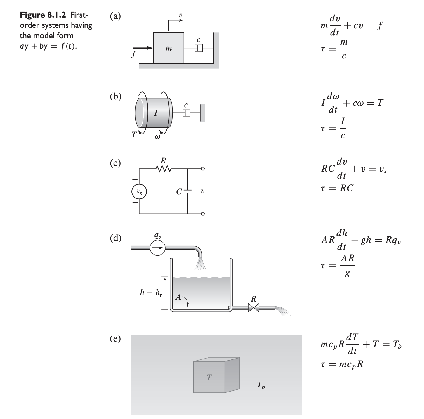
Many systems have first-order models with the same form as that of the system above, $a\dot{y}+by=f(t)$ or $\frac{a}{b}\dot{y}+y=\frac{1}{b}f(t)$.

Examples of First-Order Models

Free Response

The free response or zero input response of the model is its solution in the absence of an input. It can be obtained by using the Laplace transform:

$$m[sV(s)-v(0^{-})]+cV(s)=F(s)$$

Then, since this is the free response, we have $f(t)=0$. This gives us:

$$\begin{array}{rl}m\dot{v}+cv& =0\\ msV(s)-mv(0)+cV(s)& =0\\ msV(s)+cV(s)& =mv(0)\\ V(s)& =\frac{mv(0)}{ms+c}=\frac{v(0)}{s+\frac{c}{m}}\end{array}$$

which gives:

$$v(t)=v(0)e^{-\frac{c}{m}t}$$

where $v(0)$ is the initial value of the response $v(t)$, and $m$ and $c$ are constants.

• When $c/m<0$ the solution grows exponentially; this is the unstable case.
• If $c/m=0$, the model is neutrally stable, and $v(t)=v(0)$.
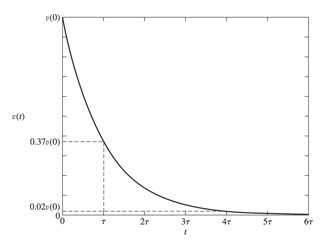
• If $c/m$ is positive, the model is stable, and the solution decays exponentially.

For the stable case, we can introduce a time constant:

$$\tau =\frac{m}{c}$$

and re-write the equation above as:

$$v(t)=v(0)e^{-t/\tau }$$

Forced Response

In the forced response case, we have

$$\begin{array}{rl}msV(s)-mv(0)+cV(s)& =F(s)\\ V(s)(ms+c)& =F(s)+mv(0)\\ V(s)& =\underset{\text{ZSR}}{\underbrace{\frac{F(s)}{ms+c}}}+\underset{\text{ZIR}}{\underbrace{\frac{mv(0)}{ms+c}}}\end{array}$$

where the ZSR is the zero-state response and ZIR is the zero-input response.

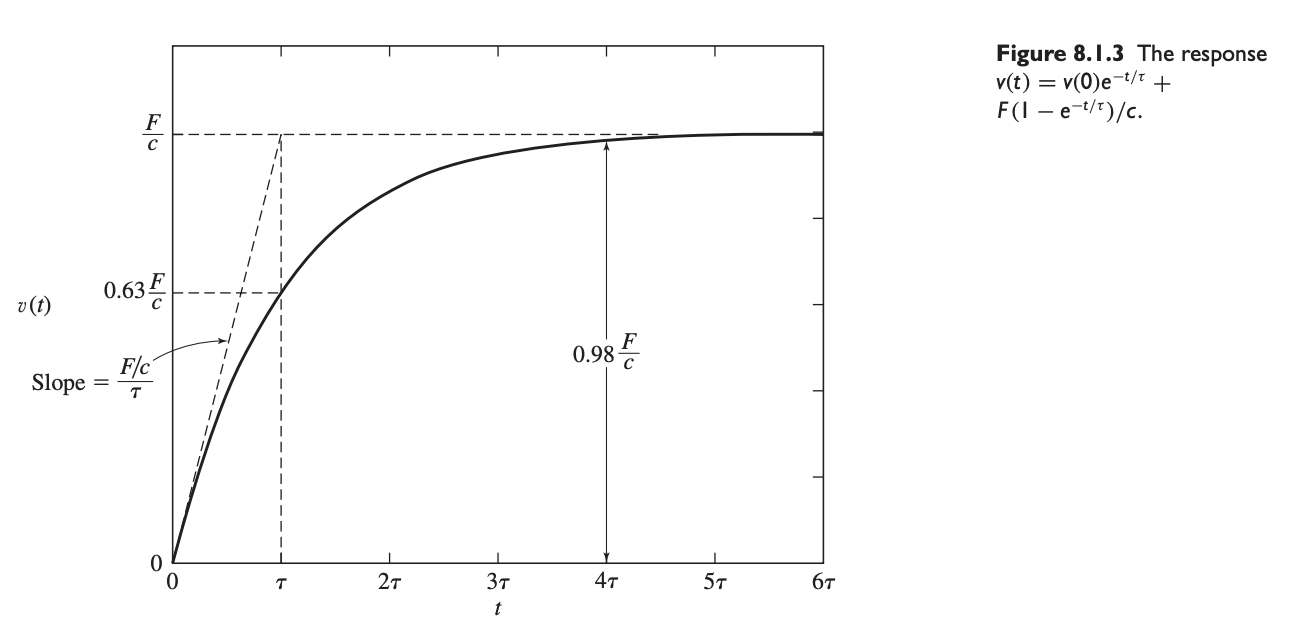
Step Response

In the case of a step input, we have

$$f(t)=Fu(t)$$

Recall that $\mathcal{L}\{u(t)\}=\frac{1}{s}$, so we have

$$F(s)=\frac{F}{s}$$

So we have:

$$m[sV(s)-v(0)]+cV(s)=\frac{F}{s}$$

where $F$ is the magnitude of the step input.

Solving for $V(s)$:

$$\begin{array}{rl}V(s)& =\frac{mv(0)}{ms+c}+\frac{F}{s(ms+c)}\\ & =\frac{v(0)}{s+c/m}+\frac{F}{c}\left(\frac{1}{s}-\frac{1}{s+c/m}\right)\end{array}$$

which in turn gives:

$$\begin{array}{rl}v(t)& =\underset{\text{Free response}}{\underbrace{v(0)e^{-\frac{c}{m}t}}}+\underset{\text{Forced response}}{\underbrace{\frac{F}{c}\left(1-e^{-\frac{c}{m}t}\right)}}\end{array}$$

Transient vs Steady-State Response

We can also arrange the terms above to get:

$$v(t)=\underset{\text{Transient response}}{\underbrace{\left(v(0)-\frac{F}{c}\right)e^{-\frac{c}{m}t}}}+\underset{\text{SS response}}{\underbrace{\frac{F}{c}}}$$

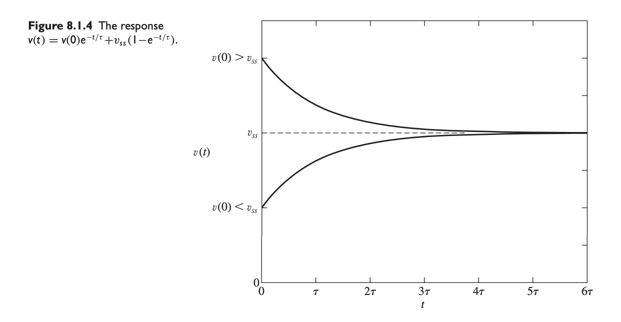
The transient response term eventually disappears as $t$ increases, while the steady-state (SS) response term stays.

• In the above, $v_{ss}=\frac{F}{C}$.
• Basically what the above graph tells us no matter the starting $v(0)$, it will eventually converge to $v(t)=v_{ss}$ because of the transient term disappearing.