Instrumentation Amplifiers

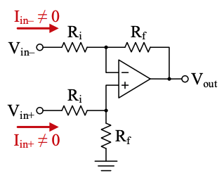
Basic op-amp circuits suffer from two significant drawbacks when configured as difference amplifiers.

• First, the difference amplifier requires current on both its input terminals. However, many sensors cannot deliver current and must be connected to high-impedance amplifier inputs. Though modern op-amps usually require minimal input current, the difference amplifier circuit relies on a current balance in the feedback path on the negative input and a voltage divider on the positive input. -
• Secondly, mismatches in the $R_i$ and $R_f$ resistors coupled with the op-amp’s own CMRR can quickly lead to an unacceptable overall CMRR.

Instrumentation Amplifiers

An instrumentation amplifier solves these problems by buffering the input signals and using well-matched resistors.

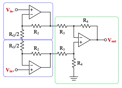
Stage 1 (blue) consists of two non-inverting op-amp configurations whose primary purpose is to to buffer the input.

• $R_G$ is a single resistor intended to set the gain, whereas all the other resistors are fixed values. $R_G$ is divided in half to help visualize Stage 1 as a non-inverting configuration. The node between the two halves of $R_G$ acts as a virtual ground when a differential signal is applied since the upper and lower Stage 1 amplifiers move symmetrically about that voltage. Visualize the fulcrum in a seesaw – the voltage should remain constant.

Stage 2 (green) is simply a difference amplifier.

The gain is:

$$A_d=A_1{A}_2=\left(1+\frac{R_2}{R_G/2}\right)\frac{R_4}{R_3}$$

If $R_2=R_3=R_4=R$, then the gain simplifies to:

$$A_d=1+\frac{2R}{R_G}$$

If $R_G$ deviates from its intended value through component tolerance, drift, or sensitivity to operating conditions, the positive and negative gains are symmetrically impacted. So, though $A_d$ changes due to errors in $R_G$, $A_{cm}$ will not, leading to a far better CMRR than using separate Stage 1 gain resistors.

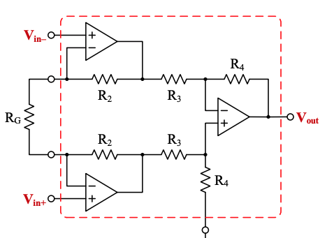
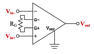
In integrated circuit (IC) form, the boundary would be shown in red. $R_G$ would be user-supplied, and $V_{in+}$, $V_{in-}$ and $V_{out}$ would be exposed terminals. The voltage divider ground terminal would also be exposed as $V_{ref}$, which can set the DC offset of the output signal. the symbol for an instrumentation amplifiers is sometimes drawn as shown.