UDL Chapter 7 Problems

Problem 7.1

A two-layer network with two hidden units in each layer can be defined as:

$$\begin{array}{rl}y={\varphi }_0& +{\varphi }_{1}a[{\psi }_{01}+{\psi }_{11}a[{\theta }_{01}+{\theta }_{11}x]+{\psi }_{21}a[{\theta }_{02}+{\theta }_{12}x]]\\ & +{\varphi }_{2}a[{\psi }_{02}+{\psi }_{12}a[{\theta }_{01}+{\theta }_{11}x]+{\psi }_{22}a[{\theta }_{02}+{\theta }_{12}x]]\end{array}$$

where the functions $a[\bullet ]$ are ReLU functions. Compute the derivatives of the output $y$ with respect to each of the 13 parameters ${\varphi }_{\bullet },{\theta }_{\bullet \bullet }$ and ${\psi }_{\bullet \bullet }$ directly. The derivatives of the ReLU function with respect to its input $\partial a[z]/\partial [z]$ is the indicator function $\mathbb{I}[z>0]$, which returns one if the argument is greater than zero and zero otherwise.

Output layer:

$$\begin{array}{rl}\frac{\partial y}{\partial {\varphi }_0}& =1\\ \frac{\partial y}{\partial {\varphi }_1}& =a[{\psi }_{01}+{\psi }_{11}a[{\theta }_{01}+{\theta }_{11}x]+{\psi }_{21}a[{\theta }_{02}+{\theta }_{12}x]]\\ \frac{\partial y}{\partial {\varphi }_2}& =a[{\psi }_{02}+{\psi }_{12}a[{\theta }_{01}+{\theta }_{11}x]+{\psi }_{22}a[{\theta }_{02}+{\theta }_{12}x]]\end{array}$$

Second hidden layer: Let us first define

$$\begin{array}{r}{h}_{21}={\psi }_{01}+{\psi }_{11}\cdot a[z_1]+{\psi }_{21}\cdot a[z_2]\\ h_{22}={\psi }_{02}+{\psi }_{12}\cdot a[z_1]+{\psi }_{22}\cdot a[z_2]\end{array}$$

Then:

$$\begin{array}{rl}\frac{\partial y}{\partial {\psi }_{01}}& =\frac{\partial y}{\partial a[h_{21}]}\frac{\partial a[h_{21}]}{\partial h_{21}}\frac{\partial {\psi }_{01}}{\partial h_{21}}={\varphi }_1\cdot \mathbb{I}(h_{21}>0)\cdot 1\\ \frac{\partial y}{\partial {\psi }_{11}}& =\frac{\partial y}{\partial a[h_{21}]}\frac{\partial a[h_{21}]}{\partial h_{21}}\frac{\partial {\psi }_{11}}{\partial h_{21}}={\varphi }_1\cdot \mathbb{I}(h_{21}>0)\cdot a[{\theta }_{01}+{\theta }_{11}x]\\ \frac{\partial y}{\partial {\psi }_{21}}& =\frac{\partial y}{\partial a[h_{21}]}\frac{\partial a[h_{21}]}{\partial h_{21}}\frac{\partial {\psi }_{21}}{\partial h_{21}}={\varphi }_1\cdot \mathbb{I}(h_{21}>0)\cdot a[{\theta }_{02}+{\theta }_{12}x]\\ \frac{\partial y}{\partial {\psi }_{02}}& =\frac{\partial y}{\partial a[h_{22}]}\frac{\partial a[h_{22}]}{\partial h_{22}}\frac{\partial {\psi }_{02}}{\partial h_{22}}={\varphi }_2\cdot \mathbb{I}(h_{22}>0)\cdot 1\\ \frac{\partial y}{\partial {\psi }_{12}}& =\frac{\partial y}{\partial a[h_{22}]}\frac{\partial a[h_{22}]}{\partial h_{22}}\frac{\partial {\psi }_{12}}{\partial h_{22}}={\varphi }_2\cdot \mathbb{I}(h_{22}>0)\cdot a[{\theta }_{01}+{\theta }_{11}x]\\ \frac{\partial y}{\partial {\psi }_{22}}& =\frac{\partial y}{\partial a[h_{22}]}\frac{\partial a[h_{22}]}{\partial h_{22}}\frac{\partial {\psi }_{22}}{\partial h_{22}}={\varphi }_2\cdot \mathbb{I}(h_{22}>0)\cdot a[{\theta }_{02}+{\theta }_{12}x]\end{array}$$

First hidden layer: Let us first define

$$\begin{array}{r}{h}_{11}={\theta }_{01}+{\theta }_{11}x\\ h_{12}={\theta }_{02}+{\theta }_{12}x\end{array}$$

Then we have:

$$\begin{array}{rl}\frac{\partial y}{\partial {\theta }_{01}}& =\frac{\partial y}{\partial a[h_{21}]}\frac{\partial a[h_{21}]}{\partial h_{21}}\frac{\partial h_{21}}{\partial a[h_{11}]}\frac{\partial a[h_{11}]}{\partial h_{11}}\frac{\partial h_{11}}{\partial {\theta }_{01}}\\ & ={\varphi }_1\cdot \mathbb{I}(h_{21}>0)\cdot {\psi }_{11}\cdot \mathbb{I}(h_{11}>0)\cdot 1\\ \frac{\partial y}{\partial {\theta }_{11}}& =\frac{\partial y}{\partial a[h_{21}]}\frac{\partial a[h_{21}]}{\partial h_{21}}\frac{\partial h_{21}}{\partial a[h_{11}]}\frac{\partial a[h_{11}]}{\partial h_{11}}\frac{\partial h_{11}}{\partial {\theta }_{11}}\\ & ={\varphi }_1\cdot \mathbb{I}(h_{21}>0)\cdot {\psi }_{11}\cdot \mathbb{I}(h_{11}>0)\cdot x\\ \frac{\partial y}{\partial {\theta }_{02}}& =\frac{\partial y}{\partial a[h_{22}]}\frac{\partial a[h_{22}]}{\partial h_{22}}\frac{\partial h_{22}}{\partial a[h_{12}]}\frac{\partial a[h_{12}]}{\partial h_{12}}\frac{\partial h_{12}}{\partial {\theta }_{02}}\\ & ={\varphi }_2\cdot \mathbb{I}(h_{22}>0)\cdot {\psi }_{12}\cdot \mathbb{I}(h_{12}>0)\cdot 1\\ \frac{\partial y}{\partial {\theta }_{12}}& =\frac{\partial y}{\partial a[h_{22}]}\frac{\partial a[h_{22}]}{\partial h_{22}}\frac{\partial h_{22}}{\partial a[h_{12}]}\frac{\partial a[h_{12}]}{\partial h_{12}}\frac{\partial h_{12}}{\partial {\theta }_{12}}\\ & ={\varphi }_2\cdot \mathbb{I}(h_{22}>0)\cdot {\psi }_{12}\cdot \mathbb{I}(h_{12}>0)\cdot x\end{array}$$

Problem 7.2

Find an expression for the final term in each of the five chains of derivatives in equation 7.13.

$$\begin{array}{rl}\frac{\partial {\ell }_i}{\partial f_2}& =\left(\frac{\partial {\ell }_i}{\partial f_3}\frac{\partial f_3}{\partial h_3}\right)\frac{\partial h_3}{\partial f_2}\\ & =2(f_3-y_i)\cdot {\omega }_3\cdot -\sin f_2\end{array}$$ $$\begin{array}{rl}\frac{\partial {\ell }_i}{\partial h_2}& =\left(\frac{\partial {\ell }_i}{\partial f_3}\frac{\partial f_3}{\partial h_3}\frac{\partial h_3}{\partial f_2}\right)\frac{\partial f_2}{\partial h_2}\\ & =2(f_3-y_i)\cdot {\omega }_3\cdot -\sin f_2\cdot {\omega }_2\end{array}$$ $$\begin{array}{rl}\frac{\partial {\ell }_i}{\partial f_1}& =\left(\frac{\partial {\ell }_i}{\partial f_3}\frac{\partial f_3}{\partial h_3}\frac{\partial h_3}{\partial f_2}\frac{\partial f_2}{\partial h_2}\right)\frac{\partial h_2}{\partial f_1}\\ & =2(f_3-y_i)\cdot {\omega }_3\cdot -\sin f_2\cdot {\omega }_2\cdot \exp [f_1]\end{array}$$ $$\begin{array}{rl}\frac{\partial {\ell }_i}{\partial h_1}& =\left(\frac{\partial {\ell }_i}{\partial f_3}\frac{\partial f_3}{\partial h_3}\frac{\partial h_3}{\partial f_2}\frac{\partial f_2}{\partial h_2}\frac{\partial h_2}{\partial f_1}\right)\frac{\partial f_1}{\partial h_1}\\ & =2(f_3-y_i)\cdot {\omega }_3\cdot -\sin f_2\cdot {\omega }_2\cdot \exp [f_1]\cdot {\omega }_1\end{array}$$ $$\begin{array}{rl}\frac{\partial {\ell }_i}{\partial f_0}& =\left(\frac{\partial {\ell }_i}{\partial f_3}\frac{\partial f_3}{\partial h_3}\frac{\partial h_3}{\partial f_2}\frac{\partial f_2}{\partial h_2}\frac{\partial h_2}{\partial f_1}\frac{\partial f_1}{\partial h_1}\right)\frac{\partial h_1}{\partial f_0}\\ & =2(f_3-y_i)\cdot {\omega }_3\cdot -\sin f_2\cdot {\omega }_2\cdot \exp [f_1]\cdot {\omega }_1\cdot \cos [f_0]\end{array}$$

Problem 7.3

What size are each of the terms in equation 7.20?

• $\frac{\partial {\mathbf{f}}_2}{\partial {\mathbf{h}}_2}$ is $D_3\times D_2$
• $\frac{\partial {\mathbf{h}}_2}{\partial {\mathbf{f}}_1}$ is $D_2\times D_2$
• $\frac{\partial {\mathbf{f}}_1}{\partial {\mathbf{h}}_1}$ is $D_2\times D_1$
• $\frac{\partial {\mathbf{h}}_1}{\partial {\mathbf{f}}_0}$is $D_1\times D_1$

Problem 7.4

Calculate the derivative $\frac{\partial {\ell }_i}{\partial \text{f}[{\mathbf{x}}_i,\varphi ]}$ for the least squares loss function:

$${\ell }_i=(y_i-\text{f}[{\mathbf{x}}_i,\varphi ]{)}^2$$

$$\frac{\partial {\ell }_i}{\partial \text{f}[{\mathbf{x}}_i,\varphi ]}=2(y_i-\text{f}[{\mathbf{x}}_i,\varphi ])(-1)=2(\text{f}[{\mathbf{x}}_i,\varphi ]-y_i)$$

Problem 7.5

Calculate the derivative $\frac{\partial {\ell }_i}{\partial \text{f}[{\mathbf{x}}_i,\varphi ]}$ for the binary classification loss function:

$${\ell }_i=-(1-y_i)\log [1-\text{sig}[\text{f}[{\mathbf{x}}_i,\varphi ]\left]\right]-y_i\log \left[\text{sig}\right[\text{f}[{\mathbf{x}}_i,\varphi ]\left]\right]$$

For the sake of clean math let’s write $f=\text{f}[{\mathbf{x}}_i,\varphi ]$. So we want to find $\frac{\partial {\ell }_i}{\partial f}$.

We have:

$$\frac{\partial {\ell }_i}{\partial f}=\frac{\partial {\ell }_i}{\partial \text{sig}[f]}\frac{\partial \text{sig}[f]}{\partial f}$$

The first term is:

$$\begin{array}{rl}\frac{\partial {\ell }_i}{\partial \text{sig}[f]}& =-(1-y_i)\left(\frac{1}{1-\text{sig}[f]}\right)(-1)-(y_i)\left(\frac{1}{\text{sig}[f]}\right)(1)\\ & =\frac{1-y_i}{1-\text{sig}[f]}-\frac{y_i}{\text{sig}[f]}\end{array}$$

The second term is:

$$\frac{\partial \text{sig}[f]}{\partial f}=\frac{\exp [-f]}{(1+\exp [-f]{)}^2}$$

Combining them back, we have:

$$\frac{\partial {\ell }_i}{\partial f}=\left(\frac{1-y_i}{1-\text{sig}\left[f\right]}-\frac{y_i}{\text{sig}[f]}\right)\left(\frac{\exp [-f]}{(1+\exp [-f]{)}^2}\right)$$

Recall that the sigmoid is:

$$\begin{array}{rl}\text{sig}[f]& =\frac{1}{1+\exp [-f]}\\ 1-\text{sig}[f]& =\frac{\exp [-f]}{1+\exp [-f]}\end{array}$$

Let’s substitute these back into our loss function and simplify:

\begin{align} \frac{ \partial \ell_{i} }{ \partial f } & = \left( (1-y_{i}) \left( \frac{1+\exp[-f]}{\exp[-f]} \right) - (y_{i}) (1+\exp[-f]) \right) \left( \frac{\exp[-f]}{(1+\exp[-f])^{2}} \right) \\[2ex] & = \left( \frac{(1-y_{i})(1+\exp[-f])}{\exp[-f]} - (y_{i}) (1+\exp[-f])\right)\left( \frac{\exp[-f]}{(1+\exp[-f])^{2}} \right) \\[2ex] & =\cancel{ (1+\exp[-f]) }\left( \frac{1-y_{i}}{\exp[-f]} - y_{i} \right)\left( \frac{\exp[-f]}{(1+\exp[-f])^\cancel{ {2} }} \right)\\[2ex] & =\left( \frac{1-y_{i}}{\exp[-f]}-y_{i} \right)\left( \frac{\exp[-f]}{1+\exp[-f]} \right) \\[2ex] & = \frac{1-y_{i}}{1+\exp[-f]}-\frac{y_{i}\exp[-f]}{1+\exp[-f]} \\[2ex] & = \frac{1-y_{i}-y_{i}\exp[-f]}{1+\exp[-f]} \\[2ex] & = \frac{1}{1+\exp[-f]}- \frac{y_{i}+y_{i}\exp[-f]}{1+\exp[-f]} \\[2ex] & = \frac{1}{1+\exp[-f]}-\frac{y_{i}(1+\exp[-f])}{1+\exp[-f]} \\[2ex] & = \frac{1}{1+\exp[-f]} - y_{i} \\[2ex] & =\boxed{\text{sig}[f]-y_{i}} \end{align}

Nice result (and seems important)!

Problem 7.6

Show that for $\mathbf{z}=\beta +\mathbf{\Omega h}$:

$$\frac{\partial \mathbf{z}}{\partial \mathbf{h}}={\mathbf{\Omega }}^T$$

where $\partial \mathbf{z}/\partial \mathbf{h}$ is a matrix containing the term $\partial z_i/\partial h_j$ in its $i$-th column and $j$-th row.

To do this, first find an expression for the constituent elements $\partial z_i/\partial h_j$, and then consider the form that the matrix $\partial \mathbf{z}/\partial \mathbf{h}$ must take.

Let:

$$\mathbf{h}=\left[\begin{array}{c}{h}_1\\ ⋮\\ h_n\end{array}\right],\mathbf{z}=\beta +\Omega \mathbf{h},\mathbf{\Omega }=[{\Omega }_{ij}]\in {\mathbb{R}}^{m\times n}$$

so that $z_i={\beta }_i+{\sum }_{k=1}^n{\mathbf{\Omega }}_{ik}{h}_k$. We can see this is in action in Example Computation – ${\mathbf{\Omega }}_{ik}{\mathbf{h}}_k$ is a dot product between $\mathbf{h}$ and the $i$-th row of $\Omega$, and then we add the bias for that row.

Now let’s consider the element-wise derivative. For some fixed $i$ and $j$:

$$\frac{\partial z_i}{\partial h_j}=\frac{\partial }{\partial h_j}\left({\beta }_i+\sum _k{\mathbf{\Omega }}_{ik}{h}_k\right)={\mathbf{\Omega }}_{ij}$$

This is because $z_i$ depends linearly on each $h_j$, so the partial derivative just plucks out the corresponding weight.

Then, since $\partial \mathbf{z}/\partial \mathbf{h}$ is a matrix containing the term $\partial z_i/\partial h_j$ in its $i$-th column and $j$-th row”:

$$\frac{\partial \mathbf{z}}{\partial \mathbf{h}}={\left[\frac{\partial z_i}{\partial h_j}\right]}_{\text{row }j,\text{col }i}={\Omega }_{ij}$$

Now we can notice that the matrix whose $(j,i)$ entry is ${\Omega }_{ij}$ is precisely the transpose of $\mathbf{\Omega }$, leading us to:

$$\frac{\partial \mathbf{z}}{\partial \mathbf{h}}={\mathbf{\Omega }}^T$$

If you instead store instead in row $i$, column $j$ —the more common “Jacobian” convention—the matrix would be $\mathbf{\Omega }$ itself. The textbook’s row/column choice therefore introduces the transpose.

Problem 7.7

Consider the case where we use the logistic sigmoid as an activation function, so $h=\text{sig}[f]$. Compute the derivative $\partial h/\partial f$ for this activation function. What happens to the derivative when the input takes (i) a large positive value and (ii) a large negative value?

We have:

$$h=\text{sig}[f]=\frac{1}{1+\exp [-f]}$$

and it follows that

$$\frac{\partial h}{\partial f}=\frac{\partial \text{sig}[f]}{\partial f}=\frac{\exp [-f]}{(1+\exp [-f]{)}^2}$$

which can then be re-written as:

$$\begin{array}{rl}\frac{\partial h}{\partial f}& =\frac{1}{1+\exp [-f]}\cdot \frac{\exp [-f]}{1+\exp [-f]}\\ & =\text{sig}[f]\cdot (1-\text{sig}[f])\\ & =h(1-h)\end{array}$$

When the input $f$ becomes large positive value, $h=\text{sig}[f]\approx 1$, so we have $1(1-1)=0$. When the input $f$ becomes a large negative value, we in turn have $h\approx 0$, which gives $0(1-0)=0$. Thus, the gradient is (near) zero at both extremes.

Problem 7.8

Consider using (i) the Heaviside function and (ii) the rectangular function as activations:

$$\text{Heaviside}[z]=\{\begin{array}{ll}0& z<0\\ 1& z\ge 0\end{array}$$ $$\text{rect}[z]=\{\begin{array}{ll}0& z<0\\ 1& 0\le z\le 1\\ 0& z>1\end{array}$$

Discuss why these functions are problematic for neural network training with gradient-based optimization methods.

Both of these functions are flat and discontinuous.

In regions where the function is flat, weights before the activation will not change because the chain rule will include a multiplication by zero. For some weight $w$:

$$\frac{\partial L}{\partial w}=\frac{\partial L}{\partial a}\cdot \frac{\partial a}{\partial z}\cdot \frac{\partial z}{\partial w}$$

In this case $\frac{\partial a}{\partial z}=0$ because the activation is flat, so we also just have $\frac{\partial L}{\partial w}=0$ and the weight doesn’t update at all.

In regions where the function is discontinuous, there’s no gradient to follow (undefined) – optimization algorithms like gradient descent are stuck.

Problem 7.9

Consider a loss function $\ell [\mathbf{f}]$, where $\mathbf{f}=\beta +\mathbf{\Omega h}$. We want to find how the loss $\ell$ changes when we change $\mathbf{\Omega }$, which we’ll express with a matrix that contains the derivative $\partial \ell /\partial {\Omega }_{ij}$ at the $i$-th row and $j$-th column. Find an expression for $\partial f_i/\partial {\Omega }_{ij}$, and, using the chain rule, show that

$$\frac{\partial \ell }{\partial \Omega }=\frac{\partial \ell }{\partial \mathbf{f}}{\mathbf{h}}^T$$

We have

$$f_i={\beta }_i+\sum _j{\mathbf{\Omega }}_{ij}{h}_j$$

and so:

$$\frac{\partial f_i}{\partial {\mathbf{\Omega }}_{ij}}=h_j$$

Using the chain rule:

$$\frac{\partial \ell }{\partial {\mathbf{\Omega }}_{ij}}=\frac{\partial \ell }{\partial f_i}\frac{\partial f_i}{\partial {\mathbf{\Omega }}_{ij}}=\frac{\partial \ell }{\partial f_i}{h}_j$$

Converting back to vector form, we have

$$\frac{\partial \ell }{\partial \mathbf{\Omega }}=\frac{\partial \ell }{\partial \mathbf{f}}{\mathbf{h}}^T$$

as required.

Problem 7.10

Derive the equations for the backward pass of the backpropagation algorithm that uses leaky ReLU activations, which are defined as:

$$\mathbf{a}[z]=\text{ReLU}[z]=\{\begin{array}{ll}\alpha \cdot z& z<0\\ z& z\ge 0\end{array}$$

where $\alpha$ is a small positive constant, typically $0.1$.

The Leaky ReLU has a gradient of $+1$ when the input is greater than zero, and a gradient of $\alpha$ when the gradient is less than zero. The backprop equations are the same except for

$$\frac{\partial {\ell }_i}{\partial {\mathbf{f}}_{k-1}}=\mathbb{I}[{\mathbf{f}}_{k-1}>0]\odot \left({\mathbf{\Omega }}_k^T\frac{\partial {\ell }_i}{\partial {\mathbf{f}}_{\mathbf{k}}}\right)+\mathbb{I}[{\mathbf{f}}_{\mathbf{k}-1}<0]\odot \alpha \left({\mathbf{\Omega }}_k^T\frac{\partial {\ell }_i}{\partial {\mathbf{f}}_k}\right)$$

Problem 7.11

Consider training a network with fifty layers, where we only have enough memory to store the pre-activations at every tenth hidden layer during the forward pass. Explain how to compute the derivatives in this situation using gradient checkpointing.

We just start from each 10th hidden layers.

• We have the loss gradient at 50 and the saved checkpoint at 40, so we recompute the forward for layers 41-50 from the saved state at 40. Then we backprop through 50 to 41, accumulating parameter grads and the gradient wrt the activation at layer 40.
• Then we just move to the next window - recompute forward 31 to 40, 21–30, 11–20, and 1–10,

Problem 7.12

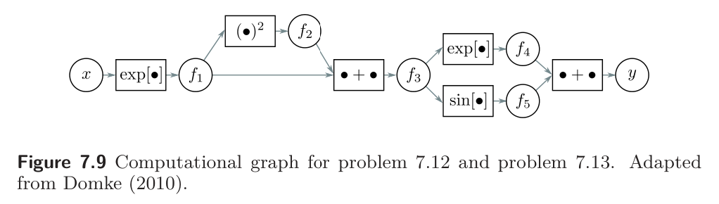
This problem explores computing derivatives on general acyclic computational graphs. Consider the function:

$$y=\exp [\exp [x]+\exp [x{]}^2]+\sin [\exp [x]+\exp [x{]}^2]$$

We can break this down into a series of intermediate computations so that:

$$\begin{array}{rl}{f}_1& =\exp [x]\\ f_2& =f_1^2\\ f_3& =f_1+f_2\\ f_4& =\exp [f_3]\\ f_5& =\sin [f_3]\\ y& =f_4+f_5\end{array}$$

The associated computational graph is shown below.

Compute the derivative $\partial y/\partial x$ by reverse-mode differentiation. In other words, compute in order:

$$\frac{\partial y}{\partial f_5},\frac{\partial y}{\partial f_4},\frac{\partial y}{\partial f_3},\frac{\partial y}{\partial f_2},\frac{\partial y}{\partial f_1},\frac{\partial y}{\partial x}$$

using the chain rule in each case to make use of the derivatives already computed.

$$\begin{array}{rl}\frac{\partial y}{\partial f_5}& =1\\ \frac{\partial y}{\partial f_4}& =1\\ \frac{\partial y}{\partial f_3}& =\frac{\partial y}{\partial f_4}\frac{\partial f_4}{\partial f_3}+\frac{\partial y}{\partial f_5}\frac{\partial f_5}{\partial f_3}=\cos [f_3]+\exp [f_3]\\ \frac{\partial y}{\partial f_2}& =\frac{\partial y}{\partial f_3}\frac{\partial f_3}{\partial f_2}=\cos [f_3]+\exp [f_3]\\ \frac{\partial y}{\partial f_1}& =\frac{\partial y}{\partial f_3}\frac{\partial f_3}{\partial f_1}+\frac{\partial y}{\partial f_3}\frac{\partial f_2}{\partial f_1}=\cos [f_3]+\exp [f_3]+(\cos [f_3]+\exp [f_3])(2f_1)\\ \frac{\partial y}{\partial x}& =\frac{\partial y}{\partial f_1}\frac{\partial f_1}{\partial x}=\exp [x](\cos [f_3]+\exp [f_3]+(\cos [f_3]+\exp [f_3])(2f_1))\end{array}$$

Problem 7.13

For the same function as 7.12, compute the derivative $\partial y/\partial x$ by forward-mode differentiation. In other words, compute in order:

$$\frac{\partial f_1}{\partial x},\frac{\partial f_2}{\partial x},\frac{\partial f_3}{\partial x},\frac{\partial f_4}{\partial x},\frac{\partial f_5}{\partial x},\frac{\partial y}{\partial x}$$

using the chain rule in each case to make use of the derivatives already computed. Why do we not use forward-mode differentiation when we calculate the parameter gradients for deep networks?

$$\begin{array}{rl}\frac{\partial f_1}{\partial x}& =\exp [x]\\ \frac{\partial f_2}{\partial x}& =\frac{\partial f_2}{\partial f_1}\frac{\partial f_1}{\partial x}=2f_1\exp [x]\\ \frac{\partial f_3}{\partial x}& =\frac{\partial f_3}{\partial f_1}\frac{\partial f_1}{\partial x}+\frac{\partial f_3}{\partial f_2}\frac{\partial f_2}{\partial x}=\exp [x]+2f_1\exp [x]=\exp [x](1+2f_1)\\ \frac{\partial f_4}{\partial x}& =\frac{\partial f_4}{\partial f_3}\frac{\partial f_3}{\partial x}=\exp [f_3]\exp [x](1+2f_1)\\ \frac{\partial f_5}{\partial x}& =\frac{\partial f_5}{\partial f_3}\frac{\partial f_3}{\partial x}=\cos [f_3]\exp [x](1+2f_1)\\ \frac{\partial y}{\partial x}& =\frac{\partial y}{\partial f_4}\frac{\partial f_4}{\partial x}+\frac{\partial y}{\partial f_5}\frac{\partial f_5}{\partial x}=\exp [f_3]\exp [x](1+2f_1)+\cos [f_3]\exp [x](1+2f_1)\\ & =\exp [x]((\exp [f_3]+\cos [f_3])(1+2f_1))\\ & =\exp [x](\exp [f_3]+\cos [f_3]+2f_1(\exp [f_3]+\cos [f_3]))\end{array}$$

We don’t do forward mode differentiation because for each input variable we will need to do a pass, whereas for backward mode we will have to do a pass for each output variable. Generally neural networks have fewer outputs (usually just a scalar loss) than inputs, so backward mode is cheaper.

Example with two input variables

Let’s tweak Problem 7.12 graph to have two inputs $x$ and $z$ while keeping the same structure:

$$\begin{array}{rl}{f}_1& =e^x\\ f_2& =f_1^2\\ f_3& =f_1+f_2+z(\text{new: direct input }z)\\ f_4& =e^{f_3}\\ f_5& =\sin (f_3)\\ y& =f_4+f_5\end{array}$$

Forward mode needs one pass per input:

• Pass 1 (derivatives with respect to $x$):

$$\begin{array}{rl}{\dot{f}}_1& =e^x\dot{x}=e^x\\ {\dot{f}}_2& =2f_1{\dot{f}}_1=2f_1{e}^x\\ {\dot{f}}_3& ={\dot{f}}_1+{\dot{f}}_2+\dot{z}=e^x+2f_1{e}^x=e^x(1+2f_1)\\ {\dot{f}}_4& =e^{f_3}{\dot{f}}_3\\ {\dot{f}}_5& =\cos (f_3){\dot{f}}_3\\ \dot{y}& =(e^{f_3}+\cos f_3){\dot{f}}_3=(e^{f_3}+\cos f_3)e^x(1+2f_1)=\frac{\partial y}{\partial x}\end{array}$$

• Pass 2 (derivatives with respect to $z$):

$$\begin{array}{rl}{\dot{f}}_1& =0,{\dot{f}}_2=0\\ {\dot{f}}_3& =0+0+1=1\\ {\dot{f}}_4& =e^{f_3}\\ {\dot{f}}_5& =\cos (f_3)\\ \dot{y}& =e^{f_3}+\cos f_3=\frac{\partial y}{\partial z}\end{array}$$

Reverse mode only requires one pass:

$$\begin{array}{rl}\frac{\partial y}{\partial f_5}& =1,\frac{\partial y}{\partial f_4}=1\\ \frac{\partial y}{\partial f_3}& =\frac{\partial y}{\partial f_4}\frac{\partial f_4}{\partial f_3}•\frac{\partial y}{\partial f_5}\frac{\partial f_5}{\partial f_3}=e^{f_3}+\cos f_3\\ \frac{\partial y}{\partial f_2}& =\frac{\partial y}{\partial f_3}\cdot 1=e^{f_3}+\cos f_3\\ \frac{\partial y}{\partial f_1}& =\frac{\partial y}{\partial f_3}\cdot 1•\frac{\partial y}{\partial f_2}\cdot (2f_1)=(e^{f_3}+\cos f_3)(1+2f_1)\\ \frac{\partial y}{\partial x}& =\frac{\partial y}{\partial f_1}\cdot \frac{\partial f_1}{\partial x}=(e^{f_3}+\cos f_3)(1+2f_1)e^x\\ \frac{\partial y}{\partial z}& =\frac{\partial y}{\partial f_3}\cdot \frac{\partial f_3}{\partial z}=e^{f_3}+\cos f_3\end{array}$$

Problem 7.14

Consider a random variable $a$ with variance $\text{Var}[a]={\sigma }^2$ and a symmetrical distribution around the mean $\mathbb{E}[a]=0$. Prove that if we pass this variable through the ReLU function

$$b=\text{ReLU}[a]=\{\begin{array}{ll}0& a<0\\ a& a\ge 0\end{array}$$

then the second moment of the transformed variable is $\mathbb{E}[b^2]={\sigma }^2/2$.

We have:

$$b^2=a^2{1}_{\{a\ge 0\}}$$

where $1$ is an indicator function that returns 1 is the condition inside the brackets is true and 0 if false.

Then:

$$\mathbb{E}[b^2]=\mathbb{E}[a^2{1}_{\{a\ge 0\}}]$$

To find this, let’s try to first find an expression for $\mathbb{E}[a^2]$ in terms of $\mathbb{E}[a^2{1}_{\{a\ge 0\}}]$.

Since $a$ is symmetric around 0, we have:

$$\mathbb{E}[a^2{1}_{\{a<0\}}]=\mathbb{E}[a^2{1}_{\{a\ge 0\}}]$$

Splitting $\mathbb{E}[a^2]$ into positive and negative parts:

$$\mathbb{E}[a^2]=\mathbb{E}[a^2{1}_{\{a<0\}}]+\mathbb{E}[a^2{1}_{\{a\ge 0\}}]=2\mathbb{E}[a^2{1}_{\{a\ge 0\}}]$$

Therefore,

$$\mathbb{E}[b^2]=\mathbb{E}[a^2{1}_{\{a\ge 0\}}]=\frac{1}{2}\mathbb{E}[a^2]$$

Since $\mathbb{E}[a]=0,\mathbb{E}[a^2]=\text{Var}(a)={\sigma }^2$. Thus,

$$E[b^2]=\frac{1}{2}{\sigma }^2$$

as desired.

Problem 7.15

What would you expect to happen if we initialized all of the weights and biases in the network to zero?

During gradient descent, we calculate how each neuron in a layer affects the loss. However, if all the weights are initialized to zero, all the neurons in the same layer have identical gradients; while they will update so that they are not zero, they will all update the same way.

If neurons in a layer are clones, they compute the same function, so the network loses its ability to learn different features. The output will stay the same forever.

Problem 7.16

see github

Problem 7.17

see github