Backpropagation Algorithm

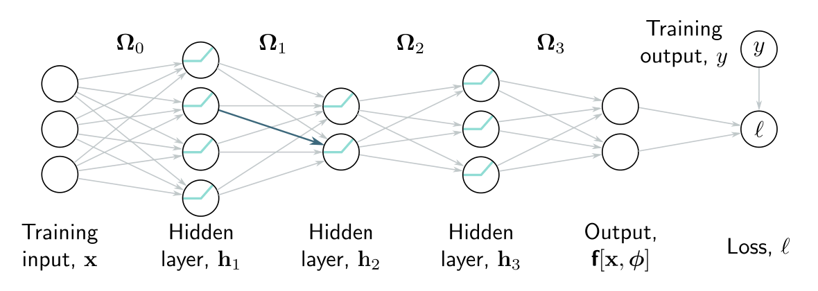
Let’s repeat the backpropagation toy example but for a three-layer network.

The intuition and much of the algebra are identical. The main differences are that intermediate variables ${\mathbf{f}}_k,{\mathbf{h}}_k$ are vectors, the biases ${\beta }_k$ are vectors, the weights ${\Omega }_k$ are matrices, and we are using ReLU functions rather than simple algebraic functions like $\cos [\bullet ]$.

Forward pass

We write the network as a series of sequential calculations:

$$\begin{array}{rl}{\mathbf{f}}_0& ={\beta }_0+{\Omega }_0{\mathbf{x}}_i\\ {\mathbf{h}}_1& =\mathbf{a}[{\mathbf{f}}_0]\\ {\mathbf{f}}_1& ={\beta }_1+{\Omega }_1{\mathbf{h}}_1\\ {\mathbf{h}}_2& =\mathbf{a}[{\mathbf{f}}_1]\\ {\mathbf{f}}_2& ={\beta }_2+{\Omega }_2{\mathbf{h}}_2\\ {\mathbf{h}}_3& =\mathbf{a}[{\mathbf{f}}_2]\\ {\mathbf{f}}_3& ={\beta }_3+{\Omega }_3{\mathbf{h}}_3\\ {\ell }_i& =\text{l}[{\mathbf{f}}_3,y_i]\end{array}$$

where:

• ${\mathbf{f}}_{k-1}$ represents the pre-activations at the $k$-th hidden layer (values before the ReLU function $\mathbf{a}[\bullet ]$)
• ${\mathbf{h}}_k$ represents the activations at the $k$-th layer (after the ReLU function)
• The term $\text{l}[{\mathbf{f}}_3,y_i]$ represents the loss function

In the forward pass, we work through these calculations and store all the intermediate values.

Backward pass 1

Now, let’s consider how the loss changes when the pre-activations ${\mathbf{f}}_0,{\mathbf{f}}_1,{\mathbf{f}}_2$ change. Applying the chain rule, the expression for the derivative of the loss with ${\ell }_i$ with respect to ${\mathbf{f}}_2$ is:

$$\frac{\partial {\ell }_i}{\partial {\mathbf{f}}_2}=\frac{\partial {\ell }_i}{\partial {\mathbf{f}}_3}\frac{\partial {\mathbf{f}}_3}{\partial {\mathbf{h}}_3}\frac{\partial {\mathbf{h}}_3}{\partial {\mathbf{f}}_2}$$

• The first term on the right has size $D_f\times 1$
  • $D_f$ is the dimension of the model output ${\mathbf{f}}_3$
• The second term has size $D_3\times D_f$
  • $D_3$ is the number of hidden units in the third layer
• The third term has size $D_3\times D_3$

Similarly, we can compute how the loss changes when we change ${\mathbf{f}}_1$ and ${\mathbf{f}}_0$:

$$\begin{array}{rl}\frac{\partial {\ell }_i}{\partial {\mathbf{f}}_1}& =\left(\frac{\partial {\ell }_i}{\partial {\mathbf{f}}_3}\frac{\partial {\mathbf{f}}_3}{\partial {\mathbf{h}}_3}\frac{\partial {\mathbf{h}}_3}{\partial {\mathbf{f}}_2}\right)\frac{\partial {\mathbf{f}}_2}{\partial {\mathbf{h}}_2}\frac{\partial {\mathbf{h}}_2}{\partial {\mathbf{f}}_1}\\ \frac{\partial {\ell }_i}{\partial {\mathbf{f}}_0}& =\left(\frac{\partial {\ell }_i}{\partial {\mathbf{f}}_3}\frac{\partial {\mathbf{f}}_3}{\partial {\mathbf{h}}_3}\frac{\partial {\mathbf{h}}_3}{\partial {\mathbf{f}}_2}\frac{\partial {\mathbf{f}}_2}{\partial {\mathbf{h}}_2}\frac{\partial {\mathbf{h}}_2}{\partial {\mathbf{f}}_1}\right)\frac{\partial {\mathbf{f}}_1}{\partial {\mathbf{h}}_1}\frac{\partial {\mathbf{h}}_1}{\partial {\mathbf{f}}_0}\end{array}$$

• In each case, the term in brackets was computed in the previous step. By working backward through the network, we can reuse previous computations.

Each term tends to be fairly simple:

• $\frac{\partial {\ell }_i}{\partial {\mathbf{f}}_3}$ (derivative of the loss ${\ell }_i$ w.r.t network output ${\mathbf{f}}_3$) depends on the loss function but generally has a simple form
• $\frac{\partial {\mathbf{f}}_3}{\partial {\mathbf{h}}_3}$ of the network output with respect to hidden layer ${\mathbf{h}}_3$ is: $$\frac{\partial {\mathbf{f}}_3}{\partial {\mathbf{h}}_3}=\frac{\partial }{\partial {\mathbf{h}}_3}({\beta }_3+{\Omega }_3{\mathbf{h}}_3)={\Omega }_3^T$$ This is shown in Problem 7.6.
• The derivative $\frac{\partial {\mathbf{h}}_3}{\partial {\mathbf{f}}_2}$ of the output ${\mathbf{h}}_3$ of the activation function with respect to its input ${\mathbf{f}}_2$ will depend on the activation function.
  • It will be a diagonal matrix since each activation only depends on the corresponding pre-activation.
  • For ReLU functions, the diagonal terms are zero everywhere ${\mathbf{f}}_2$ is less than zero and one otherwise. Rather than multiply by this matrix, we extract the diagonal terms as a vector $\mathbb{I}({\mathbf{f}}_2>0)$ and pointwise multiply, which is more efficient.

Backward pass 2

Now that we know how to compute $\frac{\partial {\ell }_i}{\partial {\mathbf{f}}_k}$, we can focus on calculating the erivatives of the loss with respect to the weights and biases.

To calculate the derivatives of the loss with respect to biases ${\beta }_k$, we use the chain rule:

$$\begin{array}{rl}\frac{\partial {\ell }_i}{\partial {\beta }_k}& =\frac{\partial {\ell }_i}{\partial {\mathbf{f}}_k}\frac{\partial {\mathbf{f}}_k}{\partial {\beta }_k}\\ & =\frac{\partial {\ell }_i}{\partial {\mathbf{f}}_k}\frac{\partial }{\partial {\beta }_k}({\beta }_k+{\Omega }_k{\mathbf{h}}_k)\\ & =\frac{\partial {\ell }_i}{\partial {\mathbf{f}}_k}\end{array}$$

which we already calculated above.

Similarly, the derivative of the weights matrix ${\Omega }_k$ is given by:

$$\begin{array}{rl}\frac{\partial {\ell }_i}{\partial {\Omega }_k}& =\frac{\partial {\ell }_i}{\partial {\mathbf{f}}_k}\frac{\partial {\mathbf{f}}_k}{\partial {\Omega }_k}\\ & =\frac{\partial {\ell }_i}{\partial {\mathbf{f}}_k}\frac{\partial }{\partial {\Omega }_k}({\beta }_k+{\Omega }_k{\mathbf{h}}_k)\\ & =\frac{\partial {\ell }_i}{\partial {\mathbf{f}}_k}{\mathbf{h}}_k^T\end{array}$$

• The progression from line 2 to 3 is shown in Problem 7.9 .

The result above makes intuitive sense; the final line is a matrix of the same size as ${\Omega }_k$. It depends linearly on ${\mathbf{h}}_k$, which was multiplied by ${\Omega }_k$ in the original expression.

This is consistent with the intuition that the derivatives of the weights in ${\Omega }_k$ will be proportional to the values of the hidden units ${\mathbf{h}}_k$ that they multiply. Recall that we already computed these during the forward pass.