Synapses

We’ve seen how individual neurons react to their input. That input usually comes from other neurons. When a neuron fires, an action potential (wave of electrical activity) travels along its axon. The junction where one neuron communicates with another is called a synapse.

A pre-synaptic action potential causes the release of a neurotransmitter, which binds to the receptors of the post-synaptic neuron, opening ion channels and thereby changing the membrane potential.

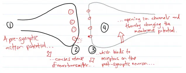
Neurons are separated by microscopic small space called the synaptic cleft, which is around 20-50mm wide.

Post-Synaptic Current

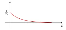
Even though an action potential is very fast, the synaptic processes by which it affects the next neuron take time. Some synapses are fast (~10ms), and some are slow (~300ms). If we represent that time constant using ${\tau }_s$,l then the current entering the post-synaptic neuron can be written as:

$$h(t)=\{\begin{array}{llc}k{t}^n{e}^{\frac{-t}{{\tau }_s}}& \text{if }t\ge 0& \text{ (for some }n\in {\mathbb{Z}}_{\ge 0})\\ 0& \text{if }t<0& \end{array}$$

where $k$ is chosen so that

$${\int }_0^{\infty }h(t)dt=1⟹k=\frac{1}{n!{\tau }_s^{n+1}}$$

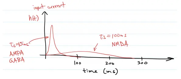
The function is called a Post-Synaptic Current (PSC) filter, or Post-Synaptic Potential (PSP) filter.

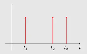
Multiple spikes form a spike train, and can be modeled as a sum of Dirac delta functions:

$$a(t)=\sum _{p=1}^3\delta (t-t_p)$$

Dirac Delta Function

The Dirac Delta Function is defined as

$$\delta (t)=\{\begin{array}{ll}\infty & \text{if }t=0\\ 0& \text{otherwise}\end{array}$$

with the properties

$${\int }_{-\infty }^{\infty }\delta (t)dt=1\text{and}{\int }_{-\infty }^{\infty }f(t)\delta (t-\tau )dt$$

The second equation there basically means that we can use the Dirac delta function that sample the value of a function at a specific $\tau$.

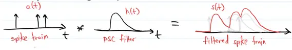
How does a spike train influence the post-synaptic neuron? We can simply add together all PSC filters, one for each spike. This is actually convolving the spike train with the PSC filter:

That is:

$$\begin{array}{rlr}s(t)& =a(t)\ast h(t)& \\ & =(a\ast h)(t)& \\ & =\left[\sum _p\delta (t-t_p)\right]\ast h(t)& \\ & =\int \sum _p\delta (\tau -t_p)h(t-\tau )d\tau & \text{[Convolution]}\\ & =\sum _{p}h(t-t_p)& \end{array}$$

which is the sum of the PSC filters, one for each spike, also known as the filtered spike train.

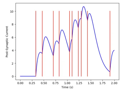
Post-synaptic current for a random spike train with ${\tau }_s,n=1$. The PSC captures some information about the pre-synaptic spike train history:

Interestingly, for a constant firing rate of $P=60\text{ Hz}$ and ${\tau }_s=0.1,n=1$, we observe that the post-synaptic current saturates to a constant value, which is determined by the pre-synaptic firing rate $P$.

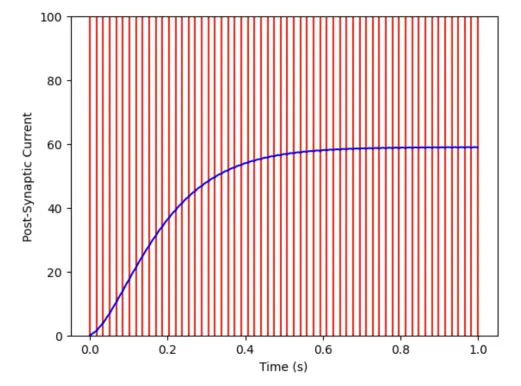
More specifically, if we plot the asymptotic value of the post-synaptic current (PSC) against the firing rate, we find a linear relationship

$$\text{PSC}\approx P$$

as demonstrated in the following plot:

Connection Weight

The total current induced by an actual potential onto a particular post-synaptic neuron can vary widely, depending on:

• The number of sizes of the synapses
• The amount and type of neurotramsitter
• The number and type of receptors

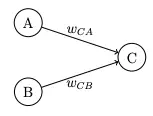
We can combine all those factors into a single number, the connection weight. Thus, the total input to a neuron is a weighted sum of filtered spike-trains.

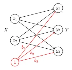
Weight Matrices

When we have many pre-synaptic neurons, it is more convenient to use matrix-vector notation to represent the weights and activities.

Suppose we have two populations $X$ and $Y$, where:

• $X$ has $N$ nodes
• $Y$ has $M$ nodes

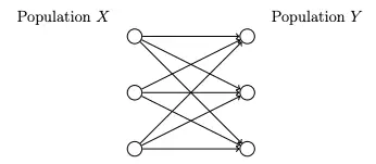
If every node in $X$ sends its output to every node in $Y$, we will have a total of $N\times M$ connections, each with its own weight.

The weights can be represented as a matrix

$$W=\left[\begin{array}{ccc}{w}_{11}& w_{12}& w_{13}\\ w_{21}& w_{22}& w_{23}\end{array}\right]$$

Vectors of Neuron Activities

We typically store the neuron activities in vectors:

$$\vec{x}=\left[\begin{array}{cc}{x}_1& x_2\end{array}\right],\vec{y}=\left[\begin{array}{ccc}{y}_1& y_2& y_3\end{array}\right]$$

We can compute the input to the nodes in $Y$ using

$$\vec{z}=\vec{x}W+b$$

where $\vec{b}$ holds the biases for the neurons in $Y$.

Thus,

$$\vec{y}=\sigma (\vec{z})=\sigma (\vec{x}W+\vec{b})$$

where $\sigma$ represents and activation function.

Bias Representation

Another way to represent the biases, $\vec{b}$, is by adding an additional input node with a fixed value of $1$.

$$\vec{x}W+\vec{b}=\left[\begin{array}{cc}\vec{x}& 1\end{array}\right]\cdot \left[\begin{array}{c}W\\ \vec{b}\end{array}\right]$$

Implementing Connections Between Spiking Neurons

For simplicity, let $n=0$:

$$h(t)=\{\begin{array}{ll}\frac{1}{{\tau }_s}{e}^{-\frac{t}{{\tau }_s}}& \text{ if }t\ge 0\\ 0& \text{if }t<0\end{array}$$

Theorem

The function $h(t)$ defined above is the solution of the initial value problem (IVP):

$${\tau }_s\frac{ds}{dt}=-s,s(0)=\frac{1}{{\tau }_s}$$

Full LIF Neuron Model

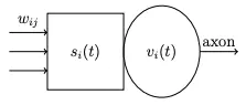
The dynamics of the neuron can be defined by:

$$\{\begin{array}{ll}{\tau }_m\frac{d{v}_i}{dt}=s_i-v_i& \text{if not in refractory period}\\ {\tau }_s\frac{d{s}_i}{dt}=-s_i& \end{array}$$

If $v_i$ reaches 1:

1. Start refractory period
2. Send spike along the axon
3. Reset $v_i$ to 0

If a spike arrives from neuron $j$: Increment $s_i$ using

$$s_i\leftarrow s_i+\frac{w_{ij}}{{\tau }_s}$$