Neural Network with Autodiff

Consider a scalar function $E$ that depends on some variable $\mathbf{v}$. Suppose we want to minimize $E$ with respect to $\mathbf{v}$, i.e.

$$\min E(\mathbf{v})$$

We can use gradient descent:

$$\mathbf{v}\leftarrow \mathbf{v}-\kappa {\nabla }_{\mathbf{v}}E(\mathbf{v})$$

where ${\nabla }_{\mathbf{v}}E(\mathbf{v})$ is the gradient of $E$ with respect to $\mathbf{v}$, and $\kappa$ is the learning rate.

Pseudocode

1. Initialize $\mathbf{v},\kappa$.
2. Construct the expression graph for $E$.
3. Until convergence:
   1. Evaluate $E$ at $\mathbf{v}$
   2. Set gradients to zero (i.e. $\mathbf{v}$.grad = 0)
   3. Propagate derivatives down (increment $\mathbf{v}$.grad)
   4. Update $\mathbf{v}\leftarrow \mathbf{v}-\kappa \cdot \mathbf{v}$.grad

Neural Learning

We use the same process to implement error propagation for neural networks, and we optimize with respect to the connection weights and biases.

To accomplish this, our network will be composed of a series of layers, each layer transforming the data from the layer below it, culminating in a scalar-valued cost function.

There are two types of operations in the network:

1. Multiply by connection weights (including adding biases)
2. Apply activation function

Finally, a cost function takes the output of the network, as well as the targets, and returns a scalar.

Let us consider this small network:

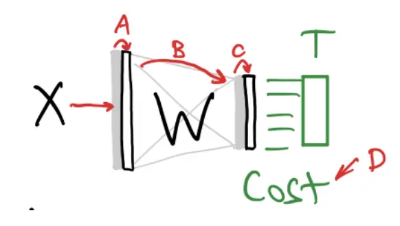
Given dataset $(X,T)$:

$$\begin{array}{rlr}A& =\text{identity}& \\ B& =(z\to z\cdot W)& (\text{multiply by }W)\\ C& =\text{logistic function}& (\text{logistic function})\\ D& =\text{Cost/loss function}& \end{array}$$

These are all functions that transform their input.

Each layer can be called like a function:

$$\begin{array}{rlr}x& =A(X)& \text{e.g,}A(X)=X\\ z& =B(x)& \text{e.g.,}B(x)=x\cdot W\\ y& =C(z)& \text{e.g.,}C(z)=\sigma (z)\\ E& =D(y,T)& \text{e.g.,}D(T,y)=\mathbb{E}\left[\frac{1}{2}{\left|\left|y-T\right|\right|}_2^2\right]\end{array}$$

Each layer, including the cost function, is just a function in a nested mathematical expression:

$$E=D(C(B(A(X))),T)$$

Neural learning is:

$$W\leftarrow W-\kappa {\nabla }_{W}E$$

We construct our network using objects from our AD classes (Variables and Operations) so that we can take advantage of their backward() methods to compute the gradients.

$$\begin{array}{rlr}\text{net}& =(A,B,C)& \\ y& =\text{net}(X)=C(B(A(x)))& \text{(Forward pass sets network state)}\\ E& =D(y,T)& \end{array}$$

Then, we take gradient steps:

E.zero_grad()
E.backward()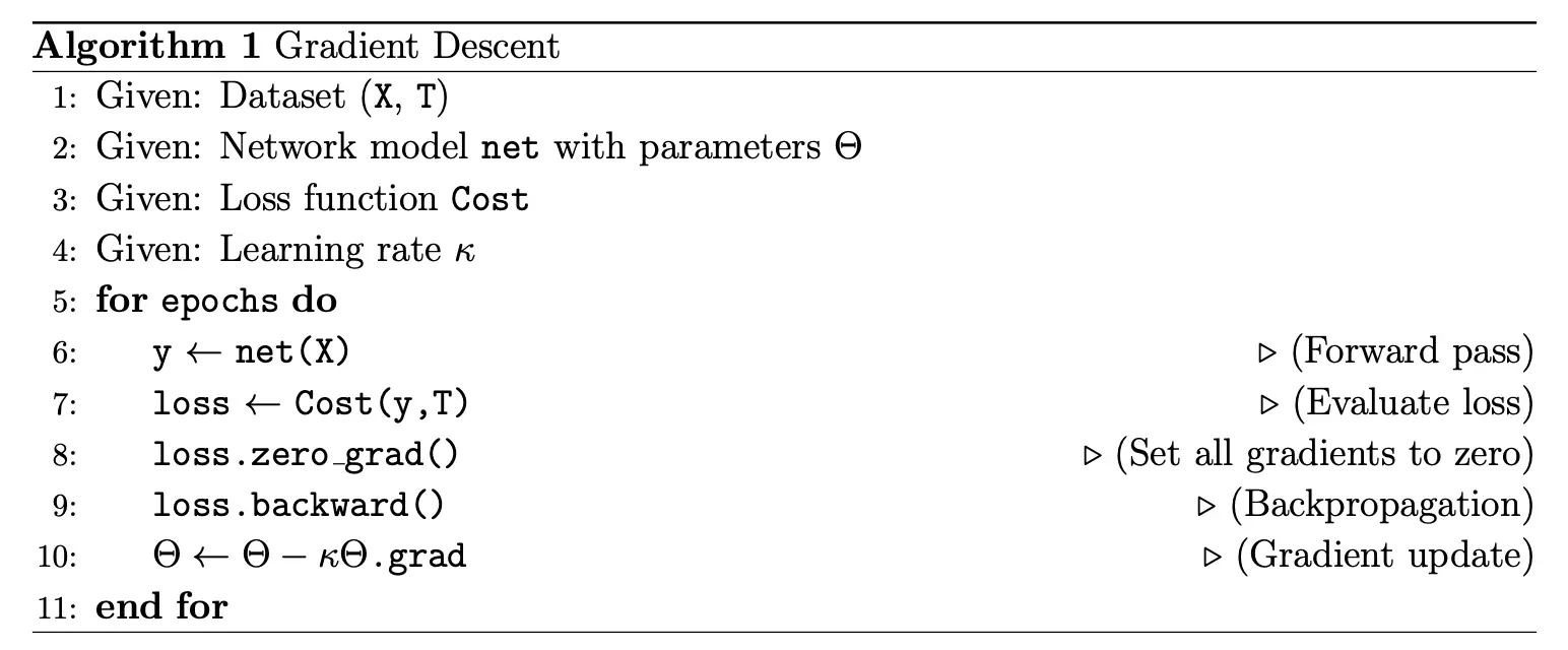

Matrix Autodiff

To work with neural networks, our AD library will have to deal with matrix operations.

Matrix Addition

Suppose our scalar function involved a matrix addition:

$$L(y)\text{ is a scalar function, where }y=A+B,A,B\in {\mathbb{R}}^{M\times N}$$

What is ${\nabla }_{A}L$ and ${\nabla }_{B}L$?

$$\begin{array}{rlr}{\nabla }_{A}L& ={\nabla }_{y}L\odot {\nabla }_{A}y=s\odot 1_{M\times N}& (\text{same shape as }A)\\ {\nabla }_{B}L& ={\nabla }_{y}L\odot {\nabla }_{B}y=s\odot 1_{M\times N}& (\text{same shape as }B)\end{array}$$

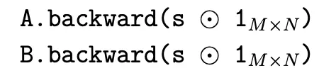
As we previously, within the plus operation method +.backward(s), we need to call the following commands

Matrix Multiplication

Suppose our scalar function involved a matrix multiplication:

$$L(\dots ,A,B,\dots ),y=A\ast B,A\in {\mathbb{R}}^{M\times N},B\in {\mathbb{R}}^{N\times K},y\in {\mathbb{R}}^{M\times K}$$

Then:

$$\begin{array}{rlr}{\nabla }_{A}L& ={\nabla }_{y}L\cdot {\nabla }_{A}y=s\cdot B^T& (M\times K\cdot K\times N\to M\times N)\\ {\nabla }_{B}L& ={\nabla }_{B}y\cdot {\nabla }_{y}L=A^T\cdot s& (N\times M\cdot M\times K\to N\times K)\end{array}$$