Leaky Integrate-and-Fire Model

The Hodgkin-Huxley Neuron Model is already vastly simplified. However, to model a single action potential takes many timesteps. However, spikes are fairly generic, and it is thought that the presence of a spike is more important than its specific shape.

Leaky Integrate-and-Fire (LIF) Model

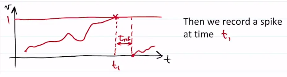
The LIF model only considers the sub-threshold membrane potential (voltage), but does NOT model the spike itself. Instead, it simply records when a spike occurs (i.e., when the voltage has reached the threshold).

$$C\frac{dV}{dt}=J_{\text{in}}-g_L(V-V_L)$$

where $C$ is a capacitance and $g_L=\frac{1}{R}$ is a conductance. The complete second term is a leak current term that is comprised of conductance multiplied by how far we are away from the equilibrium voltage. $J_{\text{in}}$ is an input current.

Multiplying everything by $R$:

$$RC\frac{dV}{dt}=R{J}_{\text{in}}-g_L(V-V_L)$$

• $RC$ term is in units of time and gets defined as $RC={\tau }_m$.
• $R{J}_{\text{in}}=V_{\text{in}}$ using Ohm’s Law

Thus, the voltage can be modeled as:

$${\tau }_m\frac{dV}{dt}=V_{\text{in}}-(V-V_L)$$

• Only valid for $V<V_{\text{th}}$ (dynamics of sub-threshold voltage)

We use a change of variables to simplify this. First, we define:

$$v=\frac{V-V_L}{V_{\text{th}}-V_L}$$

which essentially normalizes the $V$ along the entire $V_L$ to $V_{\text{th}}$ range. Then $v\to 0$ if $v_{\text{in}}=0$, and $v=1$ is the threshold.

Substituting into our differential equation, we get

$${\tau }_m\frac{dv}{dt}=v_{\text{in}}-v$$

• This has the same form as $n,h,m$ in Hodgkin-Huxley Neuron Model; it’s basically just a leaky integrator, adding up its input until it reaches equilibrium (at a rate determined by its time constant).

We integrate the differential equation for a given input current (or voltage) until $v$ reaches a threshold value of $1$. At this point we record a spike. After it spikes, it remains dormant bit for ${\tau }_{\text{ref}}$ (refractory period), and then we start integrating again from zero.

LIF Firing Rate

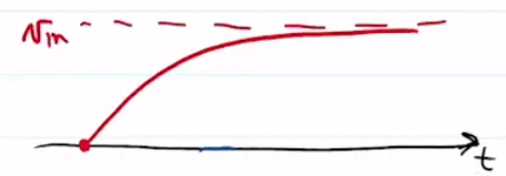
Suppose we hold the input, $v_{\text{in}}$, constant. We can solve the DE analytically between spikes. Specifically, we claim that

$$v(t)=v_{\text{in}}(1-e^{-t/\tau })$$

is a solution of $\tau \frac{dv}{dt}=v_{\text{in}}-v$, $v(0)=0$. We can prove this easily by plugging this into the equation and showing that LHS = RHS.

Visually, this will look like approaching $v_{\text{in}}$ asymptotically as $t$ increases:

Note that $v_{\text{in}}>1$, as $1$ is the threshold where we trigger a spike. After the spike, we enter the refractory period and start integrating again with the same trajectory.

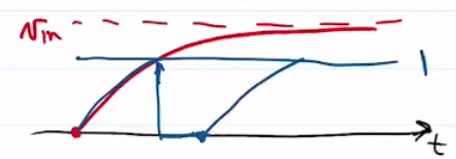
The firing rate can be found as $\frac{1}{t_{\text{isi}}}$, where $t_{\text{isi}}$ is the inter-spike interval (time between two spikes). The inter-spike interval includes the refractory period ${\tau }_{\text{ref}}$, as well as $t^{\ast }$, which is the time it takes to go from $v=0$ to $v=1$.

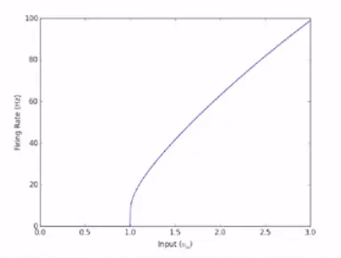
It can be shown that the steady-state firing rate for a constant input $v_{\text{in}}$ is

$$G(v_{\text{in}})=\{\begin{array}{ll}\frac{1}{{\tau }_{\text{ref}}-{\tau }_m\ln \left(1-\frac{1}{v_{\text{in}}}\right)}& \text{for }{v}_{\text{in}}>1\\ 0& \text{for }{v}_{\text{in}}\le 1\end{array}$$

The plot below shows the firing rate $G$ for various input $v_{\text{in}}$. Note again that $v_{\text{in}}>1$ for the neuron to start firing! This is called the tuning curve, which tells us how the neuron reacts to different input currents.

Typical value for cortical neurons: ${\tau }_{\text{ref}}=0.002s$, ${\tau }_m=0.02s$.