In CGP, programs are represented as directed acyclic graphs (DAG) laid out on a grid. Each node applies a function , receives inputs from earlier nodes or external inputs, and sends its output forward to later nodes.
This supports node reuse, and so the graph structure can be more compact than trees. One computed feature can feed several later computations. This makes CGP closer to digital circuits and signal-processing pipelines.
Say we want to compute . The CGP representation would be:
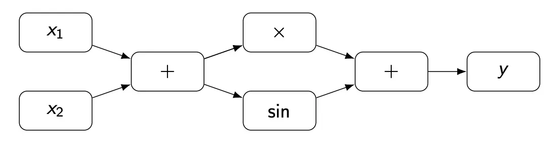
Where the node computations are:
In this, we can also see how re-using nodes works. The subexpression appears twice; but we can just compute it once as part of and then re-use it. This reduces redundancy and program size, although the genotype may still contain inactive nodes not connected to the output.
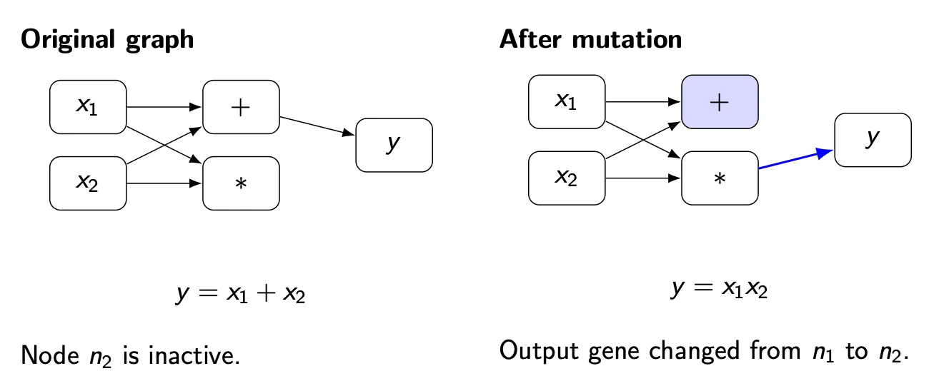
Mutation
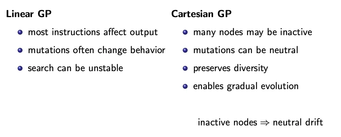
In CGP, a tiny mutation can activate a previously inactive node and change the phenotype sharply.
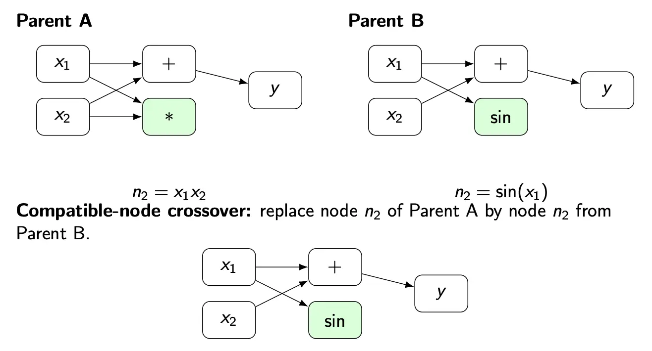
Crossover
In CGP, crossover must exchange compatible encoded nodes; arbitrary subgraph swapping an violate connectivity or acyclicity.
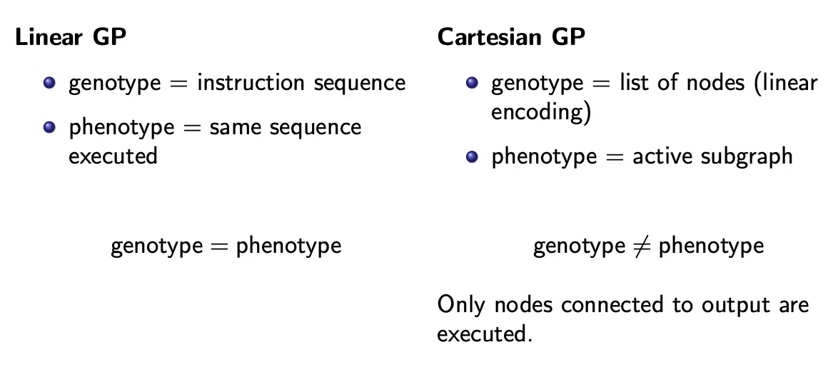
Linear vs. Cartesian GP
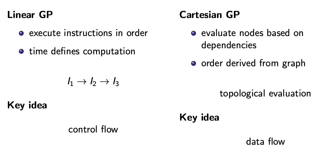
Linear GP has an implicit flow, which is made explicit in Cartesian GP. Furthermore, Cartesian GP allows for more reuse as we can reuse nodes as opposed to just registers.