Particle Filter

A particle filter represents a probability distribution with a large number of “particles” (samples). This is helpful for random variables whose pdf is unknown, so instead we draw samples.

Consider $M$ samples of the posterior $bel({\xi }_{k-1})$:

$$\Xi =\{{\xi }^{[1]},{\xi }^{[2]},\dots ,{\xi }^{[M]}\}$$

where each particle ${\xi }^{[i]}$ is a hypothesis about where the robot might be. If many particles cluster in one region, that region has high probability. If few particles appear in a region, that region has low probability.

Particle Filter Localization

We start with the previous belief distribution represented by particles:

$${\Xi }_{k-1}=\{{\xi }_{k-1}^{[1]},\dots ,{\xi }_{k-1}^{[M]}\}.$$

We apply the sample motion model to each particle to generate prediction samples to get $\overline{bel}[{\xi }_k]$

$${\xi }^{[i]}k\sim p({\xi }_k\mid {\xi }^{[i]}k-1,u_{k-1})⟶{\overline{\Xi }}_k=\{{\xi }_k^{[1]},\dots ,{\xi }_k^{[M]}\}.$$

We then do a measurement step by taking the the measurement from a (Lidar) sensor and evaluating each sample according to the sensor model:

$$w_k^{[i]}=p(z_k\mid {\xi }_k^{[i]},m)$$

where $w_k^{[i]}$ is an importance weight. This evaluates how well each particle explains the actual measurement according to the sensor.

We would then draw new samples according to importance weight $w_k^{[i]}$ to get the next estimate $bel({\xi }_k)$. This is called Importance Re-sampling with Replacement.

Importance Re-sampling

After the motion update, our particles represent the prediction distribution, $\overline{bel}({\xi }_k)$. After doing the measurement update with importance weights, our weights tell us how well each particle explains the LiDAR scan. But now, our set of particles does not match the true posterior distribution $bel({\xi }_k)$. Instead, we have samples from $\overline{bel}({\xi }_k)$ with weights that reflect how they should be redistributed.

Looking at the update rule:

$$bel({\xi }_k)=p(z_k|{\overline{\xi }}_k,m)⟹p(z_k\mid {\overline{\xi }}_k,m)=\frac{bel({\xi }_k)}{\overline{bel}({\xi }_k)}=:w_k$$

This tell us how to convert samples from $\overline{bel}$ into samples from $bel$.

Thus, if we resample the particles of $\overline{bel}({\xi }_k)$ according to the distribution of $w_k$, we should be able to recover the distribution of $bel({\xi }_k)$. Importance sampling is “resampling with replacement”; we do not change any particle’s value, we only change how frequently each one appears in the new set.

• Particles with high weight are selected many times
• Particles with low weight may disappear entirely

After this resampling, we get:

$${\Xi }_k=\{{\xi }_k^{[1]},{\xi }_k^{[2]},\dots ,{\xi }_k^{[M]}\}$$

where the distribution of particles now approximates $bel({\xi }_k)$.

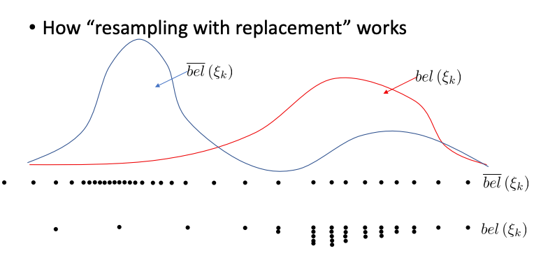
• Blue curve: Predicted distribution $\overline{bel}({\xi }_k)$ before sensor update
• Red curve: Correct posterior $bel({\xi }_k)$ after sensor update

Before resampling, the particles are spread out according to the blue curve; each particle gets a weight based on sensor likelihood. After resampling, p.articles cluster according to the red curve. Instead of explicitly shifting particles, we replicate good ones and delete bad ones.