Emulation Control Design

Two strategies of control design in DT:

1. Direct design of $D[z]$ in DT, such as IOP with SPA
   • Transient specs will be satisfied at the end of the sample points
   • Closed-loop stability at the sample points
2. Emulation design: Design $C(s)$ in CT, and then approximate $C(s)$ with $D[z]$ in DT

This is done through this series of steps. First, starting from the frequency domain $C(s)$, we use state space realization to switch to the time domain:

$$\begin{array}{rl}\dot{x}& =Ax+Be\\ u& =Cx\end{array}$$

We then use a $\Delta [k+1]$ approximation

$$\begin{array}{rl}{x}^{+}& =\hat{A}x+\hat{B}e\\ u& =Cx\end{array}$$

We then take the $Z$-transform to get to $D[z]$.

Our approximation will inevitably have some impact on the poles as we go from CT to DT.

• See Stability of CT-DT Approximation.

Approximating C(s) into D[z]

Our plan is to make an approximation in the time domain, then go back to the frequency domain.

Assume we have a continuous time system of the form:

We use a running assumption that $C(s)$ has only simple poles:

$$\begin{array}{rl}C(s)& =\sum _{i=1}^n\frac{c_i}{s-p_i}\\ & =\left[\begin{array}{ccc}1& \dots & 1\end{array}\right]\underset{=(sI-A{)}^{-1}}{\underbrace{\left[\begin{array}{ccc}\frac{1}{s-p_1}& & \\ & \ddots & \\ & & \frac{1}{s-p_n}\end{array}\right]}}\underset{B}{\underbrace{\left[\begin{array}{c}{c}_1\\ ⋮\\ c_n\end{array}\right]}}\\ & ={\left(sI-\underset{A}{\underbrace{\left[\begin{array}{ccc}{p}_1& & \\ & \ddots & \\ & & p_n\end{array}\right]}}\right)}^{-1}B\end{array}$$

Note that if we assume $d=0$, we also have

$$\begin{array}{r}U(s)=C(s)E(s)\end{array}$$

which gives

$$\begin{array}{rl}\dot{x}& =\underset{A}{\underbrace{\left[\begin{array}{ccc}{p}_1& & \\ & \ddots & \\ & & p_n\end{array}\right]}}x+\underset{B}{\underbrace{\left[\begin{array}{c}{c}_1\\ ⋮\\ c_n\end{array}\right]}}e\\ u& =\left[\begin{array}{ccc}1& \dots & 1\end{array}\right]x\end{array}$$

Recall that we can write

$$\begin{array}{rl}x[k+1]& =x[k]+\Delta [k+1]\\ & =x[k]+{\int }_{kT}^{(k+1)T}(Ax(s)+Be(s))ds\end{array}$$

We can use the left-side rule for numerical integration:

$$\begin{array}{rl}\Delta [k+1]& \approx T(Ax(kT)+Be(kT))=T(Ax[k]+Be[k])\\ & ⟹x[k+1]=x[k]+T(Ax[k]+Be[k])\end{array}$$

Taking the $z$-transform gives

$$\begin{array}{rl}zX[z]& =X[z]+T[AX[z]+BE[z]]\\ ((z-1)I-TA)X[z]& =TBE[z]\\ X[z]& =((z-1)I-TA{)}^{-1}TBE[z]\end{array}$$

We can write the $((z-1)I-TA{)}^{-1}$ term as

$$\left[\begin{array}{ccc}z-1-T{p}_1& & \\ & \ddots & \\ & & z-1-T{p}_n\end{array}\right]$$

such that we have

$$X[z]=\left[\begin{array}{c}\frac{T{c}_1}{z-1-T{p}_1}\\ ⋮\\ \frac{T{c}_n}{z-1-T{p}_n}\end{array}\right]E[z]$$

We want to find the transfer function from $U$ to $Y$:

$$u(t)=cx(t)⟶u[k]=cx[k]=\left[\begin{array}{ccc}1& \dots & 1\end{array}\right]\left[\begin{array}{c}\frac{T{c}_1}{z-1-T{p}_1}\\ ⋮\\ \frac{T{c}_n}{z-1-T{p}_n}\end{array}\right]E[z]$$

where the $[1\dots 1]$ just makes you sum all the entries in the column vector.

Thus, we have

$$U[z]=\sum _{i=1}^n\frac{T{c}_i}{z-1-T{p}_i}E[z]$$

Therefore, to get this particular approximation, we use

$$D[z]=C(s){|}_{s=\frac{1}{T}(z-1)}$$

Instead of using the left-side rule, we can take the same approach with other numerical integration methods:

With the right side rule :

$$D[z]=C(s){|}_{s=\frac{1}{T}\left(\frac{z-1}{z}\right)}$$

With the trapezoidal rule:

$$D[z]=C(s){|}_{s=\frac{2}{T}\left(\frac{z-1}{z+1}\right)}$$

Impact on Poles

Our approximation will inevitably have some impact on our poles as we go from CT to DT. Ideally, we will get stable poles in CT $⟺$ stable poles in DT.

As an example, consider this DT $D[z]$:

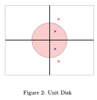
Using the left side rule with $s=\frac{1}{T}(z-1)$:

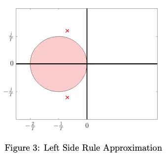
Note the location of the red poles between Figure 2 and Figure 3. Thus, for the left side rule, stable poles in CT may result in unstable poles in DT.

With the right side rule approximation $s=\frac{1}{T}\frac{z-1}{z}$:

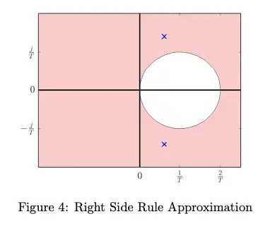
Note the location of the blue poles between Figure 2 and Figure 4. Thus, for the right side rule, unstable poles in CT may result in stable poles poles in DT.

With the trapezoidal rule $s=\frac{2}{T}\frac{z-1}{z+1}$:

Thus, for the trapezoidal rule, stable poles in CT map to stable poles in DT.

Trapezoidal approximation with a system that is closed-loop stable with $C(s)$ does not guarantee CL stability for the sampled-data system with $D[z]$. Stability of $D[z]$ does not tell us anything about closed-loop stability. This is one of the downsides of emulation design.

Step Invariant Approximation

Step invariant approximation is an emulation design method that ensures the step responses of $C(s)$ and $D[z]$ agree at sample points:

$$\begin{array}{r}{L}^{-1}\left(C(s)\frac{1}{s}\right){|}_{t=kT}=Z^{-1}\left(D[z]\frac{z}{z-1}\right)\\ ⟹D[z]=\frac{z-1}{z}Z\left(L^{-1}\left(\frac{C(s)1}{s}\right){|}_{t=kT}\right)\end{array}$$

This is the default of c2d in MATLAB.